Epidemiology is recognized both as the science basic to preventive medicine and one that informs the public health policy process. Several operational definitions of epidemiology have been suggested. The simplest is that epidemiology is the study of the occurrence of disease or other health-related characteristics in human and in animal populations. Epidemiologists study not only the frequency of disease, but whether the frequency differs across groups of people; i.e., they study the cause-effect relationship between exposure and illness. Diseases do not occur at random; they have causes—quite often man-made causes—which are avoidable. Thus, many diseases could be prevented if the causes were known. The methods of epidemiology have been crucial to identifying many causative factors which, in turn, have led to health policies designed to prevent disease, injury and premature death.

What is the task of epidemiology and what are its strengths and weaknesses when definitions and concepts of epidemiology are applied to occupational health? This chapter addresses these questions and the ways in which occupational health hazards can be investigated using epidemiological techniques. This article introduces the ideas found in successive articles in this chapter.

Occupational Epidemiology

Occupational epidemiology has been defined as the study of the effects of workplace exposures on the frequency and distribution of diseases and injuries in the population. Thus it is an exposure-oriented discipline with links to both epidemiology and occupational health (Checkoway et al. 1989). As such, it uses methods similar to those employed by epidemiology in general.

The main objective of occupational epidemiology is prevention through identifying the consequences of workplace exposures on health. This underscores the preventive focus of occupational epidemiology. Indeed, all research in the field of occupational health and safety should serve preventive purposes. Hence, epidemiological knowledge can and should be readily implementable. While the public health interest always should be the primary concern of epidemiological research, vested interests can exercise influence, and care must be taken to minimize such influence in the formulation, conduct and/or interpretation of studies (Soskolne 1985; Soskolne 1989).

A second objective of occupational epidemiology is to use results from specific settings to reduce or to eliminate hazards in the population at large. Thus, apart from providing information on the health effects of exposures in the workplace, the results from occupational epidemiology studies also play a role in the estimation of risk associated with the same exposures but at the lower levels generally experienced by the general population. Environmental contamination from industrial processes and products usually would result in lower levels of exposure than those experienced in the workplace.

The levels of application of occupational epidemiology are:

surveillance to describe the occurrence of illness in different categories of workers and so provide early warning signals of unrecognized occupational hazards

generation and testing of an hypothesis that a given exposure may be harmful, and the quantification of an effect

evaluation of an intervention (for example, a preventive action such as reduction in exposure levels) by measuring changes in the health status of a population over time.

The causal role that occupational exposures can play in the development of disease, injury and premature death had been identified long ago and is part of the history of epidemiology. Reference has to be made to Bernardino Ramazzini, founder of occupational medicine and one of the first to revive and add to the Hippocratic tradition of the dependence of health on identifiable natural external factors. In the year 1700, he wrote in his “De Morbis Artificum Diatriba” (Ramazzini 1705; Saracci 1995):

The physician has to ask many questions of the patients. Hippocrates states in De Affectionibus: “When you face a sick person you should ask him from what he is suffering, for what reason, for how many days, what he eats, and what are his bowel movements. To all these questions one should be added: ‘What work does he do?’.”

This reawakening of clinical observation and of the attention to the circumstances surrounding the occurrence of disease, brought Ramazzini to identify and describe many of the occupational diseases that were later studied by occupational physicians and epidemiologists.

Using this approach, Pott was first to report in 1775 (Pott 1775) the possible connection between cancer and occupation (Clayson 1962). His observations on cancer of the scrotum among chimney-sweeps began with a description of the disease and continued:

The fate of these people seems singularly hard: in their early infancy, they are most frequently treated with great brutality, and almost starved with cold and hunger; they are thrust up narrow, and sometimes hot chimneys, where they are bruised, burned and almost suffocated; and when they get to puberty, become peculiarly liable to a most noisome, painful, and fatal disease.

Of this last circumstance there is not the least doubt, though perhaps it may not have been sufficiently attended to, to make it generally known. Other people have cancer of the same parts; and so have others, besides lead-workers, the Poitou colic, and the consequent paralysis; but it is nevertheless a disease to which they are peculiarly liable; and so are chimney-sweeps to cancer of the scrotum and testicles.

The disease, in these people, seems to derive its origin from a lodgement of soot in the rugae of the scrotum, and at first not to be a disease of the habit … but here the subjects are young, in general good health, at least at first; the disease brought on them by their occupation, and in all probability local; which last circumstance may, I think, be fairly presumed from its always seizing the same parts; all this makes it (at first) a very different case from a cancer which appears in an elderly man.

This first account of an occupational cancer still remains a model of lucidity. The nature of the disease, the occupation concerned and the probable causal agent are all clearly defined. An increased incidence of scrotal cancer among chimney-sweeps is noted although no quantitative data are given to substantiate the claim.

Another fifty years passed before Ayrton-Paris noticed in 1822 (Ayrton-Paris 1822) the frequent development of scrotal cancers among the copper and tin smelters of Cornwall, and surmised that arsenic fumes might be the causal agent. Von Volkmann reported in 1874 skin tumours in paraffin workers in Saxony, and shortly afterwards, Bell suggested in 1876 that shale oil was responsible for cutaneous cancer (Von Volkmann 1874; Bell 1876). Reports of the occupational origin of cancer then became relatively more frequent (Clayson 1962).

Among the early observations of occupational diseases was the increased occurrence of lung cancer among Schneeberg miners (Harting and Hesse 1879). It is noteworthy (and tragic) that a recent case study shows that the epidemic of lung cancer in Schneeberg is still a huge public health problem, more than a century after the first observation in 1879. An approach to identify an “increase” in disease and even to quantify it had been present in the history of occupational medicine. For example, as Axelson (1994) has pointed out, W.A. Guy in 1843 studied “pulmonary consumption” in letter press printers and found a higher risk among compositors than among pressmen; this was done by applying a design similar to the case-control approach (Lilienfeld and Lilienfeld 1979). Nevertheless, it was not until perhaps the early 1950s that modern occupational epidemiology and its methodology began to develop. Major contributions marking this development were the studies on bladder cancer in dye workers (Case and Hosker 1954) and lung cancer among gas workers (Doll 1952).

Issues in Occupational Epidemiology

The articles in this chapter introduce both the philosophy and the tools of epidemiological investigation. They focus on assessing the exposure experience of workers and on the diseases that arise in these populations. Issues in drawing valid conclusions about possible causative links in the pathway from exposures to hazardous substances to the development of diseases are addressed in this chapter.

Ascertainment of an individual’s work life exposure experience constitutes the core of occupational epidemiology. The informativeness of an epidemiological study depends, in the first instance, on the quality and extent of available exposure data. Secondly, the health effects (or, the diseases) of concern to the occupational epidemiologist must be accurately determinable among a well-defined and accessible group of workers. Finally, data about other potential influences on the disease of interest should be available to the epidemiologist so that any occupational exposure effects that are established from the study can be attributed to the occupational exposure per se rather than to other known causes of the disease in question. For example, in a group of workers who may work with a chemical that is suspected of causing lung cancer, some workers may also have a history of tobacco smoking, a further cause of lung cancer. In the latter situation, occupational epidemiologists must determine which exposure (or, which risk factor—the chemical or the tobacco, or, indeed, the two in combination) is responsible for any increase in the risk of lung cancer in the group of workers being studied.

Exposure assessment

If a study has access only to the fact that a worker was employed in a particular industry, then the results from such a study can link health effects only to that industry. Likewise, if knowledge about exposure exists for the occupations of the workers, conclusions can be directly drawn only in so far as occupations are concerned. Indirect inferences on chemical exposures can be made, but their reliability has to be evaluated situation by situation. If a study has access, however, to information about the department and/or job title of each worker, then conclusions will be able to be made to that finer level of workplace experience. Where information about the actual substances with which a person works is known to the epidemiologist (in collaboration with an industrial hygienist), then this would be the finest level of exposure information available in the absence of rarely available dosimetry. Furthermore, the findings from such studies can provide more useful information to industry for creating safer workplaces.

Epidemiology has been a sort of “black box” discipline until now, because it has studied the relationship between exposure and disease (the two extremes of the causal chain), without considering the intermediate mechanistic steps. This approach, despite its apparent lack of refinement, has been extremely useful: in fact, all the known causes of cancer in humans, for instance, have been discovered with the tools of epidemiology.

The epidemiological method is based on available records —questionnaires, job titles or other “proxies” of exposure; this makes the conduct of epidemiological studies and the interpretation of their findings relatively simple.

Limitations of the more crude approach to exposure assessment, however, have become evident in recent years, with epidemiologists facing more complex problems. Limiting our consideration to occupational cancer epidemiology, most well-known risk factors have been discovered because of high levels of exposure in the past; a limited number of exposures for each job; large populations of exposed workers; and a clear-cut correspondence between “proxy” information and chemical exposures (e.g., shoe workers and benzene, shipyards and asbestos, and so on). Nowadays, the situation is substantially different: levels of exposure are considerably lower in Western countries (this qualification should always be stressed); workers are exposed to many different chemicals and mixtures in the same job title (e.g., agricultural workers); homogeneous populations of exposed workers are more difficult to find and are usually small in number; and, the correspondence between “proxy” information and actual exposure grows progressively weaker. In this context, the tools of epidemiology have reduced sensitivity owing to the misclassification of exposure.

In addition, epidemiology has relied on “hard” end points, such as death in most cohort studies. However, workers might prefer to see something different from “body counts” when the potential health effects of occupational exposures are studied. Therefore, the use of more direct indicators of both exposure and early response would have some advantages. Biological markers may provide just a tool.

Biological markers

The use of biological markers, such as lead levels in blood or liver function tests, is not new in occupational epidemiology. However, the utilization of molecular techniques in epidemiological studies has made possible the use of biomarkers for assessing target organ exposures, for determining susceptibility and for establishing early disease.

Potential uses of biomarkers in the context of occupational epidemiology are:

exposure assessment in cases in which traditional epidemiological tools are insufficient (particularly for low doses and low risks)

to disentangle the causative role of single chemical agents or substances in multiple exposures or mixtures

estimation of the total burden of exposure to chemicals having the same mechanistic target

investigation of pathogenetic mechanisms

study of individual susceptibility (e.g., metabolic polymorphisms, DNA repair) (Vineis 1992)

to classify exposure and/or disease more accurately, thereby increasing statistical power.

Great enthusiasm has arisen in the scientific community about these uses, but, as noted above, methodological complexity of the use of these new “molecular tools” should serve to caution against excessive optimism. Biomarkers of chemical exposures (such as DNA adducts) have several shortcomings:

They usually reflect recent exposures and, therefore, are of limited use in case-control studies, whereas they require repeated samplings over prolonged periods for utilization in cohort investigations.
While they can be highly specific and thus improve exposure misclassification, findings often remain difficult to interpret.
When complex chemical exposures are investigated (e.g., air pollution or environmental tobacco smoke) it is possible that the biomarker would reflect one particular component of the mixture, whereas the biological effect could be due to another.
In many situations, it is not clear whether a biomarker reflects a relevant exposure, a correlate of the relevant exposure, individual susceptibility, or an early disease stage, thus limiting causal inference.
The determination of most biomarkers requires an expensive test or an invasive procedure or both, thus creating constraints for adequate study size and statistical power.
A biomarker of exposure is no more than a proxy for the real objective of an epidemiological investigation, which, as a rule, focuses on an avoidable environmental exposure (Trichopoulos 1995; Pearce et al. 1995).

Even more important than the methodological shortcomings is the consideration that molecular techniques might cause us to redirect our focus from identifying risks in the exogenous environment, to identifying high-risk individuals and then making personalized risk assessments by measuring phenotype, adduct load and acquired mutations. This would direct our focus, as noted by McMichael, to a form of clinical evaluation, rather than one of public health epidemiology. Focusing on individuals could distract us from the important public health goal of creating a less hazardous environment (McMichael 1994).

Two further important issues emerge regarding the use of biomarkers:

The use of biomarkers in occupational epidemiology must be accompanied by a clear policy as far as informed consent is concerned. The worker may have several reasons to refuse cooperation. One very practical reason is that the identification of, say, an alteration in an early response marker such as sister chromatid exchange implies the possibility of discrimination by health and life insurers and by employers who might shun the worker because he or she may be more prone to disease. A second reason concerns genetic screening: since the distributions of genotypes and phenotypes vary according to ethnic group, occupational opportunities for minorities might be hampered by genetic screening. Third, doubts can be raised about the predictability of genetic tests: since the predictive value depends on the prevalence of the condition which the test aims to identify, if the latter is rare, the predictive value will be low and the practical use of the screening test will be questionable. Until now, none of the genetic screening tests have been judged applicable in the field (Ashford et al. 1990).
Ethical principles must be applied prior to the use of biomarkers. These principles have been evaluated for biomarkers used for identifying individual susceptibility to disease by an interdisciplinary Working Group of the Technical Office of the European Trade Unions, with the support of the Commission of the European Communities (Van Damme et al. 1995); their report has reinforced the view that tests can be conducted only with the objective of preventing disease in a workforce. Among other considerations, use of tests must never.

serve as a means for “selection of the fittest”

be used to avoid implementing effective preventive measures, such as the identification and substitution of risk factors or improvements in conditions in the workplace

create, confirm or reinforce social inequality

create a gap between the ethical principles followed in the workplace and the ethical principles that must be upheld in a democratic society

oblige a person seeking employment to disclose personal details other than those strictly necessary for obtaining the job.

Finally, evidence is accumulating that the metabolic activation or inactivation of hazardous substances (and of carcinogens in particular) varies considerably in human populations, and is partly genetically determined. Furthermore, inter-individual variability in the susceptibility to carcinogens may be particularly important at low levels of occupational and environmental exposure (Vineis et al. 1994). Such findings may strongly affect regulatory decisions that focus the risk assessment process on the most susceptible (Vineis and Martone 1995).

Study design and validity

Hernberg’s article on epidemiological study designs and their applications in occupational medicine concentrates on the concept of “study base”, defined as the morbidity experience (in relation to some exposure) of a population while it is followed over time. Thus, the study base is not only a population (i.e., a group of people), but the experience of disease occurrence of this population during a certain period of time (Miettinen 1985, Hernberg 1992). If this unifying concept of a study base is adopted, then it is important to recognize that the different study designs (e.g., case-control and cohort designs) are simply different ways of “harvesting” information on both exposure and disease from the same study base; they are not diametrically different approaches.

The article on validity in study design by Sasco addresses definitions and the importance of confounding. Study investigators must always consider the possibility of confounding in occupational studies, and it can never be sufficiently stressed that the identification of potentially confounding variables is an integral part of any study design and analysis. Two aspects of confounding must be addressed in occupational epidemiology:

Negative confounding should be explored: for example, some industrial populations have low exposure to lifestyle-associated risk factors because of a smoke-free workplace; glass blowers tend to smoke less than the general population.
When confounding is considered, an estimate of its direction and its potential impact ought to be assessed. This is particularly true when data to control confounding are scanty. For example, smoking is an important confounder in occupational epidemiology and it always should be considered. Nevertheless, when data on smoking are not available (as is often the case in cohort studies), it is unlikely that smoking can explain a large excess of risk found in an occupational group. This is nicely described in a paper by Axelson (1978) and further discussed by Greenland (1987). When detailed data on both occupation and smoking have been available in the literature, confounding did not seem to heavily distort the estimates concerning the association between lung cancer and occupation (Vineis and Simonato 1991). Furthermore, suspected confounding does not always introduce non-valid associations. Since investigators also are at risk of being led astray by other undetected observation and selection biases, these should receive as much emphasis as the issue of confounding in designing a study (Stellman 1987).

Time and time-related variables such as age at risk, calendar period, time since hire, time since first exposure, duration of exposure and their treatment at the analysis stage, are among the most complex methodological issues in occupational epidemiology. They are not covered in this chapter, but two relevant and recent methodological references are noted (Pearce 1992; Robins et al. 1992).

Statistics

The article on statistics by Biggeri and Braga, as well as the title of this chapter, indicate that statistical methods cannot be separated from epidemiological research. This is because: (a) a sound understanding of statistics may provide valuable insights into the proper design of an investigation and (b) statistics and epidemiology share a common heritage, and the entire quantitative basis of epidemiology is grounded in the notion of probability (Clayton 1992; Clayton and Hills 1993). In many of the articles that follow, empirical evidence and proof of hypothesized causal relationships are evaluated using probabilistic arguments and appropriate study designs. For example, emphasis is placed on estimating the risk measure of interest, like rates or relative risks, and on the construction of confidence intervals around these estimates instead of the execution of statistical tests of probability (Poole 1987; Gardner and Altman 1989; Greenland 1990). A brief introduction to statistical reasoning using the binomial distribution is provided. Statistics should be a companion to scientific reasoning. But it is worthless in the absence of properly designed and conducted research. Statisticians and epidemiologists are aware that the choice of methods determines what and the extent to which we make observations. The thoughtful choice of design options is therefore of fundamental importance in order to ensure valid observations.

Ethics

The last article, by Vineis, addresses ethical issues in epidemiological research. Points to be mentioned in this introduction refer to epidemiology as a discipline that implies preventive action by definition. Specific ethical aspects with regard to the protection of workers and of the population at large require recognition that:

Epidemiological studies in occupational settings should in no way delay preventive measures in the workplace.

Occupational epidemiology does not refer to lifestyle factors, but to situations where usually little or no personal role is played in the choice of exposure. This implies a particular commitment to effective prevention and to the immediate transmission of information to workers and the public.

Research uncovers health hazards and provides the knowledge for preventive action. The ethical problems of not carrying out research, when it is feasible, should be considered.

Notification to workers of the results of epidemiological studies is both an ethical and methodological issue in risk communication. Research in evaluating the potential impact and effectiveness of notification should be given high priority (Schulte et al. 1993).

Training in occupational epidemiology

People with a diverse range of backgrounds can find their way into the specialization of occupational epidemiology. Medicine, nursing and statistics are some of the more likely backgrounds seen among those specializing in this area. In North America, about half of all trained epidemiologists have science backgrounds, while the other half will have proceeded along the doctor of medicine path. In countries outside North America, most specialists in occupational epidemiology will have advanced through the doctor of medicine ranks. In North America, those with medical training tend to be considered “content experts”, while those who are trained through the science route are deemed “methodological experts”. It is often advantageous for a content expert to team up with a methodological expert in order to design and conduct the best possible study.

Not only is knowledge of epidemiological methods, statistics and computers needed for the occupational epidemiology speciality, but so is knowledge of toxicology, industrial hygiene and disease registries (Merletti and Comba 1992). Because large studies can require linkage to disease registries, knowledge of sources of population data is useful. Knowledge of labour and corporate organization also is important. Theses at the masters level and dissertations at the doctoral level of training equip students with the knowledge needed for conducting large record-based and interview-based studies among workers.

Proportion of disease attributable to occupation

The proportion of disease which is attributable to occupational exposures either in a group of exposed workers or in the general population is covered at least with respect to cancer in another part of this Encyclopaedia. Here we should remember that if an estimate is computed, it should be for a specific disease (and a specific site in the case of cancer), a specific time period and a specific geographic area. Furthermore, it should be based on accurate measures of the proportion of exposed people and the degree of exposure. This implies that the proportion of disease attributable to occupation may vary from very low or zero in certain populations to very high in others located in industrial areas where, for example, as much as 40% of lung cancer can be attributable to occupational exposures (Vineis and Simonato 1991). Estimates which are not based on a detailed review of well-designed epidemiological studies can, at the very best, be considered as informed guesses, and are of limited value.

Transfer of hazardous industries

Most epidemiological research is carried out in the developed world, where regulation and control of known occupational hazards has reduced the risk of disease over the past several decades. At the same time, however, there has been a large transfer of hazardous industries to the developing world (Jeyaratnam 1994). Chemicals previously banned in the United States or Europe now are produced in developing countries. For example, asbestos milling has been transferred from the US to Mexico, and benzidine production from European countries to the former Yugoslavia and Korea (Simonato 1986; LaDou 1991; Pearce et al. 1994).

An indirect sign of the level of occupational risk and of the working conditions in the developing world is the epidemic of acute poisoning taking place in some of these countries. According to one assessment, there are about 20,000 deaths each year in the world from acute pesticide intoxication, but this is likely to be a substantial underestimate (Kogevinas et al. 1994). It has been estimated that 99% of all deaths from acute pesticide poisoning occur in developing countries, where only 20% of the world’s agrochemicals are used (Kogevinas et al. 1994). This is to say that even if the epidemiological research seems to point to a reduction of occupational hazards, this might simply be due to the fact that most of this research is being conducted in the developed world. The occupational hazards may simply have been transferred to the developing world and the total world occupational exposure burden might have increased (Vineis et al. 1995).

Veterinary epidemiology

For obvious reasons, veterinary epidemiology is not directly pertinent to occupational health and occupational epidemiology. Nevertheless, clues to environmental and occupational causes of diseases may come from epidemiological studies on animals for several reasons:

The life span of animals is relatively short compared with that of humans, and the latency period for diseases (e.g., most cancers) is shorter in animals than in humans. This implies that a disease that occurs in a wild or pet animal can serve as a sentinel event to alert us to the presence of a potential environmental toxicant or carcinogen for humans before it would have been identified by other means (Glickman 1993).
Markers of exposures, such as haemoglobin adducts or levels of absorption and excretion of toxins, may be measured in wild and pet animals to assess environmental contamination from industrial sources (Blondin and Viau 1992; Reynolds et al. 1994; Hungerford et al. 1995).
Animals are not exposed to some factors which may act as confounders in human studies, and investigations in animal populations therefore can be conducted without regard to these potential confounders. For example, a study of lung cancer in pet dogs might detect significant associations between the disease and exposure to asbestos (e.g., via owners’ asbestos-related occupations and proximity to industrial sources of asbestos). Clearly, such a study would remove the effect of active smoking as a confounder.

Veterinarians talk about an epidemiological revolution in veterinary medicine (Schwabe 1993) and textbooks about the discipline have appeared (Thrusfield 1986; Martin et al. 1987). Certainly, clues to environmental and occupational hazards have come from the joint efforts of human and animal epidemiologists. Among others, the effect of phenoxyherbicides in sheep and dogs (Newell et al. 1984; Hayes et al. 1990), of magnetic fields (Reif et al. 1995) and pesticides (notably flea preparations) contaminated with asbestos-like compounds in dogs (Glickman et al. 1983) are notable contributions.

Participatory research, communicating results and prevention

It is important to recognize that many epidemiological studies in the field of occupational health are initiated through the experience and concern of workers themselves (Olsen et al. 1991). Often, the workers—those historically and/or presently exposed—believed that something was wrong long before this was confirmed by research. Occupational epidemiology can be thought of as a way of “making sense” of the workers’ experience, of collecting and grouping the data in a systematic way, and allowing inferences to be made about the occupational causes of their ill health. Furthermore, the workers themselves, their representatives and the people in charge of workers’ health are the most appropriate persons to interpret the data which are collected. They therefore should always be active participants in any investigation conducted in the workplace. Only their direct involvement will guarantee that the workplace will remain safe after the researchers have left. The aim of any study is the use of the results in the prevention of disease and disability, and the success of this depends to a large extent on ensuring that the exposed participate in obtaining and interpreting the results of the study. The role and use of research findings in the litigation process as workers seek compensation for damages caused through workplace exposure is beyond the scope of this chapter. For some insight on this, the reader is referred elsewhere (Soskolne, Lilienfeld and Black 1994).

Participatory approaches to ensuring the conduct of occupational epidemiological research have in some places become standard practice in the form of steering committees established to oversee the research initiative from its inception to its completion. These committees are multipartite in their structure, including labour, science, management and/or government. With representatives of all stakeholder groups in the research process, the communication of results will be made more effective by virtue of their enhanced credibility because “one of their own” would have been overseeing the research and would be communicating the findings to his or her respective constituency. In this way, the greatest level of effective prevention is likely.

These and other participatory approaches in occupational health research are undertaken with the involvement of those who experience or are otherwise affected by the exposure-related problem of concern. This should be seen more commonly in all epidemiological research (Laurell et al. 1992). It is relevant to remember that while in epidemiological work the objective of analysis is estimation of the magnitude and distribution of risk, in participatory research, the preventability of the risk is also an objective (Loewenson and Biocca 1995). This complementarity of epidemiology and effective prevention is part of the message of this Encyclopaedia and of this chapter.

Maintaining public health relevance

Although new developments in epidemiological methodology, in data analysis and in exposure assessment and measurement (such as new molecular biological techniques) are welcome and important, they can also contribute to a reductionist approach focusing on individuals, rather than on populations. It has been said that:

… epidemiology has largely ceased to function as part of a multidisciplinary approach to understanding the causation of disease in populations and has become a set of generic methods for measuring associations of exposure and disease in individuals.… There is current neglect of social, economic, cultural, historical, political and other population factors as major causes of diseases.…Epidemiology must reintegrate itself into public health, and must rediscover the population perspective (Pearce 1996).

Occupational and environmental epidemiologists have an important role to play, not only in developing new epidemiological methods and applications for these methods, but also in ensuring that these methods are always integrated in the proper population perspective.

Back

Published in 28. Epidemiology and Statistics

Monday, 28 February 2011 21:01

Exposure Assessment

The assessment of exposures is a critical step in identifying workplace hazards through epidemiological investigation. The exposure assessment process may be subdivided into a series of activities. These include:

compiling an inventory of potentially toxic agents and mixtures present in the targeted work environment
determining how exposures occur and how likely they are to vary among employees
selecting appropriate measures or indices for quantifying exposures
collecting data that will enable study participants to be assigned qualitative or quantitative exposure values for each measure. Whenever possible, these activities should be carried out under the guidance of a qualified industrial hygienist.

Occupational health studies are often criticized because of inadequacies in the assessment of exposures. Inadequacies may lead to differential or non-differential misclassification of exposure and subsequent bias or loss of precision in the exposure-effect analyses. Efforts to improve the situation are evidenced by several recent international conferences and texts devoted to this topic (ACGIH 1991; Armstrong et al. 1992; Proceedings of the Conference on Retrospective Assessment of Occupational Exposures in Epidemiology 1995). Clearly, technical developments are providing new opportunities for advancing exposure assessment. These developments include improvements in analytical instrumentation, a better understanding of pharmacokinetic processes, and the discovery of new biomarkers of exposure. Because occupational health studies often depend on historic exposure information for which no specific monitoring would have been undertaken, the need for retrospective exposure assessment adds an additional dimension of complexity to these studies. However, improved standards for assessment and for ensuring the reliability of such assessments continue to be developed (Siemiatycki et al. 1986). Prospective exposure assessments, of course, can be more readily validated.

The term exposure refers to the concentration of an agent at the boundary between individual and environment. Exposure is normally presumed when an agent is known to be present in a work environment and there is a reasonable expectation of employee contact with that agent. Exposures may be expressed as an 8-hour time-weighted-average (TWA) concentration, which is a measure of exposure intensity that has been averaged over an 8-hour work shift. Peak concentrations are intensities averaged over shorter time periods such as 15 minutes. Cumulative exposure is a measure of the product of average intensity and duration (e.g., a mean 8-hour TWA concentration multiplied by years worked at that mean concentration). Depending on the nature of the study and the health outcomes of interest, evaluation of peak, average intensity, cumulative or lagged exposures may be desirable.

By way of contrast, dose refers to the deposition or absorption of an agent per unit time. Dose or daily intake of an agent may be estimated by combining environmental measurement data with standard assumptions regarding, among other factors, breathing rates and dermal penetration. Alternatively, intake may be estimated based on biomonitoring data. Dose ideally would be measured at the target organ of interest.

Important exposure assessment factors include:

identification of the relevant agents
determination of their presence and concentrations in appropriate environmental media (e.g., air, contact surfaces)
assessment of the likely routes of entry (inhalation, skin absorption, ingestion), the time course of exposure (daily variation), and cumulative duration of exposure expressed in weeks, months or years
evaluation of the effectiveness of engineering and personal controls (e.g., use of protective clothing and respiratory protection may mediate exposures) and, finally
host and other considerations that may modulate target organ concentrations.

These include the physical level of work activity and the prior health status of individuals. Special care should be taken in assessing exposure to agents that are persistent or tend to bioaccumulate (e.g., certain metals, radionuclides or stable organic compounds). With these materials, internal body burdens may increase insidiously even when environmental concentrations appear to be low.

While the situation can be quite complex, often it is not. Certainly, many valuable contributions to identifying occupational hazards have come from studies using common-sense approaches to exposure assessment. Sources of information that can be helpful in identifying and categorizing exposures include:

employee interviews
employer personnel and production records (these include work records, job descriptions, facility and process histories, and chemical inventories)
expert judgement
industrial hygiene records (area, personal, and compliance monitoring, and surface wipe samples, together with health hazard or comprehensive survey reports)
interviews with long-term or retired employees and
biomonitoring data.

There are several advantages to categorizing individual exposures in as much detail as possible. Clearly, the informativeness of a study will be enhanced to the extent that the relevant exposures have been adequately described. Secondly, the credibility of the findings may be increased because the potential for confounding can be addressed more satisfactorily. For example, referents and exposed individuals will differ as to exposure status, but may also differ relative to other measured and unmeasured explanatory factors for the disease of interest. However, if an exposure gradient can be established within the study population, it is less likely that the same degree of confounding will persist within exposure subgroups, thus strengthening the overall study findings.

Job Exposure Matrices

One of the more practical and frequently used approaches to exposure assessment has been to estimate exposures indirectly on the basis of job titles. The use of job exposure matrices can be effective when complete work histories are available and there is a reasonable constancy in both the tasks and exposures associated with the jobs under study. On the broadest scale, standard industry and job title groupings have been devised from routinely collected census data or occupational data provided on death certificates. Unfortunately, the information maintained in these large record systems is often limited to the “current” or “usual” occupation. Furthermore, because the standard groupings do not take into account the conditions present in specific workplaces, they must usually be regarded as crude exposure surrogates.

For community- and registry-based case-control studies, a more detailed exposure assessment has been achieved by utilizing expert opinion to translate job history data obtained through personal interview into semi-quantitative evaluations of likely exposures to specific agents (Siemiatycki et al. 1986). Experts, such as chemists and industrial hygienists, are chosen to assist in the exposure evaluation because of their knowledge and familiarity with various industrial processes. By combining the detailed questionnaire data with knowledge of industrial processes, this approach has been helpful in characterizing exposure differences across work facilities.

The job-exposure matrix approach has also been employed successfully in industry- and company-specific studies (Gamble and Spirtas 1976). Individual job histories (a chronological listing of past department and job assignments for each employee) are often retained in company personnel files and, when available, provide a complete job history for the employees while they are working at that facility. These data may be expanded upon through personal interviews of the study participants. The next step is to inventory all job titles and department or work area designations used during the study period. These may easily range into the hundreds or even thousands within large, multi-process facilities or across companies within an industry, when production, maintenance, research, engineering, plant support services and administrative jobs are all considered over time (often several decades), allowing for changes in industrial processes. Data consolidation can be facilitated by creating a computer file of all work history records and then using edit routines to standardize job title terminology. Those jobs involving relatively homogeneous exposures can be combined to simplify the process of linking exposures to individual jobs. However, the grouping of jobs and work locations should be supported wherever possible by measurement data collected according to a sound sampling strategy.

Even with computerized work histories, retrospective linkage of exposure data to individuals can be a difficult task. Certainly, workplace conditions will be altered as technologies change, product demand shifts, and new regulations are put in place. There may also be changes in product formulations and seasonal production patterns in many industries. Permanent records may be kept regarding some changes. However, it is less likely that records will be retained regarding seasonal and other marginal process and production changes. Employees also may be trained to perform multiple jobs and then be rotated among jobs as production demands change. All of these circumstances add complexity to the exposure profiles of employees. Nevertheless, there are also work settings that have remained relatively unchanged for many years. In the final analysis, each work setting must be evaluated in its own right.

Ultimately, it will be necessary to summarize the worklife exposure history of each person in a study. Considerable influence on the final exposure-effect measures of risk has been demonstrated (Suarez-Almazor et al. 1992), and hence great care has to be exercised in selecting the most appropriate summary measure of exposure.

Industrial Hygiene—Environmental Measurement

Monitoring of work exposures is a fundamental ongoing activity in protecting employee health. Thus, industrial hygiene records may already exist at the time an epidemiological study is being planned. If so, these data should be reviewed to determine how well the target population has been covered, how many years of data are represented in the files, and how easily the measurements can be linked to jobs, work areas and individuals. These determinations will be helpful both in assessing the feasibility of the epidemiological study and in identifying data gaps that could be remedied with additional exposure sampling.

The issue of how best to link measurement data to specific jobs and individuals is a particularly important one. Area and breathing zone sampling may be helpful to industrial hygienists in identifying emission sources for corrective actions, but could be less useful in characterizing actual employee exposures unless careful time studies of employee work activities have been performed. For example, continuous area monitoring may identify excursion exposures at certain times in the day, but the question remains as to whether or not employees were in the work area at that time.

Personal sampling data generally provide more accurate estimates of employee exposure as long as the sampling is carried out under representative conditions, the use of personal protective gear is properly taken into account, and the job tasks and process conditions are relatively constant from day to day. Personal samples may be readily linked to the individual employee through the use of personal identifiers. These data may be generalized to other employees in the same jobs and to other time periods as warranted. However, based on their own experience, Rappaport et al. (1993) have cautioned that exposure concentrations may be highly variable even among employees assigned to what are considered homogeneous exposure groups. Again, expert judgement is needed in deciding whether or not homogeneous exposure groups can be presumed.

Researchers have successfully combined a job-exposure matrix approach with utilization of environmental measurement data to estimate exposures within the cells of the matrix. When measurement data are found to be lacking, it may be possible to fill in data gaps through the use of exposure modelling. Generally, this involves developing a model for relating environmental concentrations to more easily assessed determinants of exposure concentrations (e.g., production volumes, physical characteristics of the facility including the use of exhaust ventilation systems, agent volatility and nature of the work activity). The model is constructed for work settings with known environmental concentrations and then used to estimate concentrations in similar work settings lacking measurement data but having information on such parameters as constituent ingredients and production volumes. This approach may be particularly helpful for the retrospective estimation of exposures.

Another important assessment issue is the handling of exposure to mixtures. First, from an analytic viewpoint, separate detection of chemically related compounds and elimination of interferences from other substances present in the sample may not be within the capability of the analytic procedure. The various limitations in the analytic procedures used to provide measurement data need to be evaluated and the study objectives modified accordingly. Secondly, it may be that certain agents are almost always used together and hence occur in approximately the same relative proportions throughout the work environment under study. In this situation, internal statistical analyses per se will not be useful in distinguishing whether or not effects are due to one or the other agents or due to a combination of the agents. Such judgements would only be possible based on review of external studies in which the same agent combinations had not occurred. Finally, in situations where different materials are used interchangeably depending on product specifications (e.g., the use of different colourants to obtain desired colour contrasts), it may be impossible to attribute effects to any specific agent.

Biological Monitoring

Biomarkers are molecular, biochemical or cellular alterations that can be measured in biological media such as human tissue, cells or fluids. A primary reason for developing biomarkers of exposure is to provide an estimate of internal dose for a particular agent. This approach is especially useful when multiple routes of exposure are likely (e.g., inhalation and skin absorption), when protective gear is worn intermittently, or when the conditions of exposure are unpredictable. Biomonitoring can be especially advantageous when the agents of interest are known to have relatively long biological half-lives. From a statistical perspective, an advantage of biological monitoring over air monitoring may be seen with agents having a half-life as short as ten hours, depending upon the degree of environmental variability (Droz and Wu 1991). The exceedingly long half-lives of materials such as chlorinated dioxins (measured in years) make these compounds ideal candidates for biological monitoring. As with analytical methods for measuring air concentrations, one must be aware of potential interferences. For example, before utilizing a particular metabolite as a biomarker, it should be determined whether or not other common substances, such as those contained in certain medications and in cigarette smoke, could be metabolized to the same end point. In general, basic knowledge of the pharmacokinetics of an agent is needed before biological monitoring is utilized as a basis for exposure assessment.

The most frequent points of measurement include alveolar air, urine and blood. Alveolar air samples may be helpful in characterizing high short-term solvent exposures that have occurred within minutes or hours of when the sample was collected. Urinary samples are typically collected to determine excretion rates for metabolites of the compound of interest. Blood samples may be collected for direct measurement of the compound, for measurement of metabolites, or for determination of protein or DNA adducts (e.g., albumin or haemoglobin adducts, and DNA adducts in circulating lymphocytes). Accessible tissue cells, such as epithelial cells from the buccal area of the mouth, may also be sampled for identification of DNA adducts.

Determination of cholinesterase activity in red blood cells and plasma exemplifies the use of biochemical alterations as a measure of exposure. Organophosphorus pesticides inhibit cholinesterase activity and hence measurement of that activity before and after likely exposure to these compounds can be a useful indicator of exposure intensity. However, as one progresses along the spectrum of biological alterations, it becomes more difficult to distinguish between biomarkers of exposure and those of effect. In general, effect measures tend to be non-specific for the substance of interest and, therefore, other potential explanations of the effect may need to be assessed in order to support using that parameter as an exposure measure. Exposure measures should either be directly tied to the agent of interest or there should be a sound basis for linking any indirect measure to the agent. Despite these qualifications, biological monitoring holds much promise as a means for improving exposure assessment in support of epidemiological studies.

Conclusions

In making comparisons in occupational epidemiology studies, the need is to have a group of workers with exposure to compare against a group of workers without exposure. Such distinctions are crude, but can be helpful in identifying problem areas. Clearly, however, the more refined the measure of exposure, the more useful will be the study, specifically in terms of its ability to identify and develop appropriately targeted intervention programmes.

Back

Published in 28. Epidemiology and Statistics

Monday, 28 February 2011 21:03

Summary Worklife Exposure Measures

Researchers are fortunate when they have at their disposal a detailed chronology of the worklife experience of workers that provides an historic review of jobs they have held over time. For these workers a job exposure matrix can then be set up that allows each and every job change that a worker has gone through to be associated with specific exposure information.

Detailed exposure histories must be summarized for analysis purposes in order to determine whether patterns are evident that could be related to health and safety issues in the workplace. We can visualize a list of, say, 20 job changes that a worker had experienced in his or her working lifetime. There are then several alternative ways in which the exposure details (for each of the 20 job changes in this example) can be summarized, taking duration and/or concentration/dose/grade of exposure into account.

It is important to note, however, that different conclusions from a study could be reached depending on the method selected (Suarez-Almazor et al. 1992). An example of five summary worklife exposure measures is shown in table 1.

Table 1. Formulae and dimensions or units of the five selected summary measures of worklife exposure

Exposure measure	Formula	Dimensions/Units
Cumulative exposure index (CEI)	Σ (grade x time exposed)	grade and time
Mean grade (MG)	Σ (grade x time exposed)/total time exposed	grade
Highest grade ever (HG)	highest grade to which exposed for ≥ 7 days	grade
Time-weighted average (TWA) grade	Σ (grade x time exposed)/total time employed	grade
Total time exposed (TTE)	Σ time exposed	time

Adapted from Suarez-Almazor et al. 1992.

Cumulative exposure index. The cumulative exposure index (CEI) is equivalent to “dose” in toxicological studies and represents the sum, over a working lifetime, of the products of exposure grade and exposure duration for each successive job title. It includes time in its units.

Mean grade. The mean grade (MG) cumulates the products of exposure grade and exposure duration for each successive job title (i.e., the CEI) and divides by the total time exposed at any grade greater than zero. MG is independent of time in its units; the summary measure for a person exposed for a long period at a high concentration will be similar to that for a person exposed for a short period at a high concentration. Within any matched set in a case-control design, MG is an average grade of exposure per unit of time exposed. It is an average grade for the time actually exposed to the agent under consideration.

Highest grade ever. The highest grade ever (HG) is determined from scanning the work history for the highest grade assignment in the period of observation to which the worker was exposed for at least seven days. The HG could misrepresent a person’s worklife exposure because, by its very formulation, it is based on a maximizing rather than on an averaging procedure and is therefore independent of duration of exposure in its units.

Time-weighted average grade. The time-weighted average (TWA) grade is the cumulative exposure index (CEI) divided by the total time employed. Within any matched set in a case-control design, the TWA grade averages over total time employed. It differs from MG, which averages only over the total time actually exposed. Thus, TWA grade can be viewed as an average exposure per unit of time in the full term of employment regardless of exposure per se.

Total time exposed. The total time exposed (TTE) accumulates all time periods associated with exposure in units of time. TTE has appeal for its simplicity. However, it is well accepted that health effects must be related not only to duration of chemical exposure, but also to the intensity of that exposure (i.e., the concentration or grade).

Clearly, the utility of a summary exposure measure is determined by the respective weight it attributes to either duration or concentration of exposure or both. Thus different measures may produce different results (Walker and Blettner 1985). Ideally, the summary measure selected should be based on a set of defensible assumptions regarding the postulated biological mechanism for the agent or disease association under study (Smith 1987). This procedure is not, however, always possible. Very often, the biological effect of the duration of exposure or the concentration of the agent under study is unknown. In this context, the use of different exposure measures may be useful to suggest a mechanism by which exposure exerts its effect.

It is recommended that, in the absence of proved models for assessing exposure, a variety of summary worklife exposure measures be used to estimate risk. This approach would facilitate the comparison of findings across studies.

Back

Published in 28. Epidemiology and Statistics

Tuesday, 01 March 2011 01:58

Measuring Effects of Exposures

Epidemiology involves measuring the occurrence of disease and quantifying associations between diseases and exposures.

Measures of Disease Occurrence

Disease occurrence can be measured by frequencies (counts) but is better described by rates, which are composed of three elements: the number of people affected (numerator), the number of people in the source or base population (i.e., the population at risk) from which the affected persons come, and the time period covered. The denominator of the rate is the total person-time experienced by the source population. Rates allow more informative comparisons between populations of different sizes than counts alone. Risk, the probability of an individual developing disease within a specified time period, is a proportion, ranging from 0 to 1, and is not a rate per se. Attack rate, the proportion of people in a population who are affected within a specified time period, is technically a measure of risk, not a rate.

Disease-specific morbidity includes incidence, which refers to the number of persons who are newly diagnosed with the disease of interest. Prevalence refers to the number of existing cases. Mortality refers to the number of persons who die.

Incidence is defined as the number of newly diagnosed cases within a specified time period, whereas the incidence rate is this number divided by the total person-time experienced by the source population (table 1). For cancer, rates are usually expressed as annual rates per 100,000 people. Rates for other more common diseases may be expressed per a smaller number of people. For example, birth defect rates are usually expressed per 1,000 live births. Cumulative incidence, the proportion of people who become cases within a specified time period, is a measure of average risk for a population.

Table 1. Measures of disease occurrence: Hypothetical population observed for a five-year period

Newly diagnosed cases	10
Previously diagnosed living cases	12
Deaths, all causes*	5
Deaths, disease of interest	3
Persons in population	100
Years observed	5
Incidence	10 persons
Annual incidence rate
Point prevalence (at end of year 5)	(10 + 12 - 3) = 19 persons
Period prevalence (five-year period)	(10 + 12) = 22 persons
Annual death rate
Annual mortality rate

*To simplify the calculations, this example assumes that all deaths occurred at the end of the five-year period so that all 100 persons in the population were alive for the full five years.

Prevalence includes point prevalence, the number of cases of disease at a point in time, and period prevalence, the total number of cases of a disease known to have existed at some time during a specified period.

Mortality, which concerns deaths rather than newly diagnosed cases of disease, reflects factors that cause disease as well as factors related to the quality of medical care, such as screening, access to medical care, and availability of effective treatments. Consequently, hypothesis-generating efforts and aetiological research may be more informative and easier to interpret when based on incidence rather than on mortality data. However, mortality data are often more readily available on large populations than incidence data.

The term death rate is generally accepted to mean the rate for deaths from all causes combined, whereas mortality rate is the rate of death from one specific cause. For a given disease, the case-fatality rate (technically a proportion, not a rate) is the number of persons dying from the disease during a specified time period divided by the number of persons with the disease. The complement of the case-fatality rate is the survival rate. The five-year survival rate is a common benchmark for chronic diseases such as cancer.

The occurrence of a disease may vary across subgroups of the population or over time. A disease measure for an entire population, without consideration of any subgroups, is called a crude rate. For example, an incidence rate for all age groups combined is a crude rate. The rates for the individual age groups are the age-specific rates. To compare two or more populations with different age distributions, age-adjusted (or, age-standardized) rates should be calculated for each population by multiplying each age-specific rate by the per cent of the standard population (e.g., one of the populations under study, the 1970 US population) in that age group, then summing over all age groups to produce an overall age-adjusted rate. Rates can be adjusted for factors other than age, such as race, gender or smoking status, if the category-specific rates are known.

Surveillance and evaluation of descriptive data can provide clues to disease aetiology, identify high-risk subgroups that may be suitable for intervention or screening programmes, and provide data on the effectiveness of such programmes. Sources of information that have been used for surveillance activities include death certificates, medical records, cancer registries, other disease registries (e.g., birth defects registries, end-stage renal disease registries), occupational exposure registries, health or disability insurance records and workmen’s compensation records.

Measures of Association

Epidemiology attempts to identify and quantify factors that influence disease. In the simplest approach, the occurrence of disease among persons exposed to a suspect factor is compared to the occurrence among persons unexposed. The magnitude of an association between exposure and disease can be expressed in either absolute or relative terms. (See also "Case Study: Measures").

Absolute effects are measured by rate differences and risk differences (table 2). A rate difference is one rate minus a second rate. For example, if the incidence rate of leukaemia among workers exposed to benzene is 72 per 100,000 person-years and the rate among non-exposed workers is 12 per 100,000 person-years, then the rate difference is 60 per 100,000 person-years. A risk difference is a difference in risks or cumulative incidence and can range from -1 to 1.

Table 2. Measures of association for a cohort study

	Cases	Person-years at risk	Rate per 100,000
Exposed	100	20,000	500
Unexposed	200	80,000	250
Total	300	100,000	300

Rate Difference (RD) = 500/100,000 - 250/100,000

= 250/100,000 per year

(146.06/100,000 - 353.94/100,000)*

Rate ratio (or relative risk) (RR) =

Attributable risk in the exposed (AR_e) = 100/20,000 - 200/80,000

= 250/100,000 per year

Attributable risk per cent in the exposed (AR_e%) =

Population attributable risk (PAR) = 300/100,000 - 200/80,000

= 50/100,000 per year

Population attributable risk per cent (PAR%) =

* In parentheses 95% confidence intervals computed using the formulas in the boxes.

Relative effects are based on ratios of rates or risk measures, instead of differences. A rate ratio is the ratio of a rate in one population to the rate in another. The rate ratio has also been called the risk ratio, relative risk, relative rate, and incidence (or mortality) rate ratio. The measure is dimensionless and ranges from 0 to infinity. When the rate in two groups is similar (i.e., there is no effect from the exposure), the rate ratio is equal to unity (1). An exposure that increased risk would yield a rate ratio greater than unity, while a protective factor would yield a ratio between 0 and 1. The excess relative risk is the relative risk minus 1. For example, a relative risk of 1.4 may also be expressed as an excess relative risk of 40%.

In case-control studies (also called case-referent studies), persons with disease are identified (cases) and persons without disease are identified (controls or referents). Past exposures of the two groups are compared. The odds of being an exposed case is compared to the odds of being an exposed control. Complete counts of the source populations of exposed and unexposed persons are not available, so disease rates cannot be calculated. Instead, the exposed cases can be compared to the exposed controls by calculation of relative odds, or the odds ratio (table 3).

Table 3. Measures of association for case-control studies: Exposure to wood dust and adenocarcinoma of the nasal cavity and paranasal sinues

	Cases	Controls
Exposed	18	55
Unexposed	5	140
Total	23	195

Relative odds (odds ratio) (OR) =

Attributable risk per cent in the exposed () =

Population attributable risk per cent (PAR%) =

where = proportion of exposed controls = 55/195 = 0.28

* In parentheses 95% confidence intervals computed using the formulas in the box overleaf.

Source: Adapted from Hayes et al. 1986.

Relative measures of effect are used more frequently than absolute measures to report the strength of an association. Absolute measures, however, may provide a better indication of the public health impact of an association. A small relative increase in a common disease, such as heart disease, may affect more persons (large risk difference) and have more of an impact on public health than a large relative increase (but small absolute difference) in a rare disease, such as angiosarcoma of the liver.

Significance Testing

Testing for statistical significance is often performed on measures of effect to evaluate the likelihood that the effect observed differs from the null hypothesis (i.e., no effect). While many studies, particularly in other areas of biomedical research, may express significance by p-values, epidemiological studies typically present confidence intervals (CI) (also called confidence limits). A 95% confidence interval, for example, is a range of values for the effect measure that includes the estimated measure obtained from the study data and that which has 95% probability of including the true value. Values outside the interval are deemed to be unlikely to include the true measure of effect. If the CI for a rate ratio includes unity, then there is no statistically significant difference between the groups being compared.

Confidence intervals are more informative than p-values alone. A p-value’s size is determined by either or both of two reasons. Either the measure of association (e.g., rate ratio, risk difference) is large or the populations under study are large. For example, a small difference in disease rates observed in a large population may yield a highly significant p-value. The reasons for the large p-value cannot be identified from the p-value alone. Confidence intervals, however, allow us to disentangle the two factors. First, the magnitude of the effect is discernible by the values of the effect measure and the numbers encompassed by the interval. Larger risk ratios, for example, indicate a stronger effect. Second, the size of the population affects the width of the confidence interval. Small populations with statistically unstable estimates generate wider confidence intervals than larger populations.

The level of confidence chosen to express the variability of the results (the “statistical significance”) is arbitrary, but has traditionally been 95%, which corresponds to a p-value of 0.05. A 95% confidence interval has a 95% probability of containing the true measure of the effect. Other levels of confidence, such as 90%, are occasionally used.

Exposures can be dichotomous (e.g., exposed and unexposed), or may involve many levels of exposure. Effect measures (i.e., response) can vary by level of exposure. Evaluating exposure-response relationships is an important part of interpreting epidemiological data. The analogue to exposure-response in animal studies is “dose-response”. If the response increases with exposure level, an association is more likely to be causal than if no trend is observed. Statistical tests to evaluate exposure-response relationships include the Mantel extension test and the chi-square trend test.

Standardization

To take into account factors other than the primary exposure of interest and the disease, measures of association may be standardized through stratification or regression techniques. Stratification means dividing the populations into homogenous groups with respect to the factor (e.g., gender groups, age groups, smoking groups). Risk ratios or odds ratios are calculated for each stratum and overall weighted averages of the risk ratios or odds ratios are calculated. These overall values reflect the association between the primary exposure and disease, adjusted for the stratification factor, i.e., the association with the effects of the stratification factor removed.

A standardized rate ratio (SRR) is the ratio of two standardized rates. In other words, an SRR is a weighted average of stratum-specific rate ratios where the weights for each stratum are the person-time distribution of the non-exposed, or referent, group. SRRs for two or more groups may be compared if the same weights are used. Confidence intervals can be constructed for SRRs as for rate ratios.

The standardized mortality ratio (SMR) is a weighted average of age-specific rate ratios where the weights (e.g., person-time at risk) come from the group under study and the rates come from the referent population, the opposite of the situation in a SRR. The usual referent population is the general population, whose mortality rates may be readily available and based on large numbers and thus are more stable than using rates from a non-exposed cohort or subgroup of the occupational population under study. Using the weights from the cohort instead of the referent population is called indirect standardization. The SMR is the ratio of the observed number of deaths in the cohort to the expected number, based on the rates from the referent population (the ratio is typically multiplied by 100 for presentation). If no association exists, the SMR equals 100. It should be noted that because the rates come from the referent population and the weights come from the study group, two or more SMRs tend not to be comparable. This non-comparability is often forgotten in the interpretation of epidemiological data, and erroneous conclusions can be drawn.

Healthy Worker Effect

It is very common for occupational cohorts to have lower total mortality than the general population, even if the workers are at increased risk for selected causes of death from workplace exposures. This phenomenon, called the healthy worker effect, reflects the fact that any group of employed persons is likely to be healthier, on average, than the general population, which includes workers and persons unable to work due to illnesses and disabilities. The overall mortality rate in the general population tends to be higher than the rate in workers. The effect varies in strength by cause of death. For example, it appears to be less important for cancer in general than for chronic obstructive lung disease. One reason for this is that it is likely that most cancers would not have developed out of any predisposition towards cancer underlying job/career selection at a younger age. The healthy worker effect in a given group of workers tends to diminish over time.

Proportional Mortality

Sometimes a complete tabulation of a cohort (i.e., person-time at risk) is not available and there is information only on the deaths or some subset of deaths experienced by the cohort (e.g., deaths among retirees and active employees, but not among workers who left employment before becoming eligible for a pension). Computation of person-years requires special methods to deal with person-time assessment, including life-table methods. Without total person-time information on all cohort members, regardless of disease status, SMRs and SRRs cannot be calculated. Instead, proportional mortality ratios (PMRs) can be used. A PMR is the ratio of the observed number of deaths due to a specific cause in comparison to the expected number, based on the proportion of total deaths due to the specific cause in the referent population, multiplied by the number of total deaths in the study group, multiplied by 100.

Because the proportion of deaths from all causes combined must equal 1 (PMR=100), some PMRs may appear to be in excess, but are actually artificially inflated due to real deficits in other causes of death. Similarly, some apparent deficits may merely reflect real excesses of other causes of death. For example, if aerial pesticide applicators have a large real excess of deaths due to accidents, the mathematical requirement that the PMR for all causes combined equal 100 may cause some one or other causes of death to appear deficient even if the mortality is excessive. To ameliorate this potential problem, researchers interested primarily in cancer can calculate proportionate cancer mortality ratios (PCMRs). PCMRs compare the observed number of cancer deaths to the number expected based on the proportion of total cancer deaths (rather than all deaths) for the cancer of interest in the referent population multiplied by the total number of cancer deaths in the study group, multiplied by 100. Thus, the PCMR will not be affected by an aberration (excess or deficit) in a non-cancer cause of death, such as accidents, heart disease or non-malignant lung disease.

PMR studies can better be analysed using mortality odds ratios (MORs), in essence analysing the data as if they were from a case-control study. The “controls” are the deaths from a subset of all deaths that are thought to be unrelated to the exposure under study. For example, if the main interest of the study were cancer, mortality odds ratios could be calculated comparing exposure among the cancer deaths to exposure among the cardiovascular deaths. This approach, like the PCMR, avoids the problems with the PMR which arise when a fluctuation in one cause of death affects the apparent risk of another simply because the overall PMR must equal 100. The choice of the control causes of death is critical, however. As mentioned above, they must not be related to the exposure, but the possible relationship between exposure and disease may not be known for many potential control diseases.

Attributable Risk

There are measures available which express the amount of disease that would be attributable to an exposure if the observed association between the exposure and disease were causal. The attributable risk in the exposed (AR_e) is the disease rate in the exposed minus the rate in the unexposed. Because disease rates cannot be measured directly in case-control studies, the AR_e is calculable only for cohort studies. A related, more intuitive, measure, the attributable risk percent in the exposed (AR_e%), can be obtained from either study design. The AR_e% is the proportion of cases arising in the exposed population that is attributable to the exposure (see table 2 and table 3 for formula). The AR_e% is the rate ratio (or the odds ratio) minus 1, divided by the rate ratio (or odds ratio), multiplied by 100.

The population attributable risk (PAR) and the population attributable risk per cent (PAR%), or aetiological fraction, express the amount of disease in the total population, which is comprised of exposed and unexposed persons, that is due to the exposure if the observed association is causal. The PAR can be obtained from cohort studies (table 28.3 ) and the PAR% can be calculated in both cohort and case-control studies (table 2 and table 3).

Representativeness

There are several measures of risk that have been described. Each assumes underlying methods for counting events and in the representatives of these events to a defined group. When results are compared across studies, an understanding of the methods used is essential for explaining any observed differences.

Back

Published in 28. Epidemiology and Statistics

Tuesday, 01 March 2011 01:48

Options in Study Design

The epidemiologist is interested in relationships between variables, chiefly exposure and outcome variables. Typically, epidemiologists want to ascertain whether the occurrence of disease is related to the presence of a particular agent (exposure) in the population. The ways in which these relationships are studied may vary considerably. One can identify all persons who are exposed to that agent and follow them up to measure the incidence of disease, comparing such incidence with disease occurrence in a suitable unexposed population. Alternatively, one can simply sample from among the exposed and unexposed, without having a complete enumeration of them. Or, as a third alternative, one can identify all people who develop a disease of interest in a defined time period (“cases”) and a suitable group of disease-free individuals (a sample of the source population of cases), and ascertain whether the patterns of exposure differ between the two groups. Follow-up of study participants is one option (in so-called longitudinal studies): in this situation, a time lag exists between the occurrence of exposure and disease onset. One alternative option is a cross-section of the population, where both exposure and disease are measured at the same point in time.

In this article, attention is given to the common study designs—cohort, case-referent (case-control) and cross-sectional. To set the stage for this discussion, consider a large viscose rayon factory in a small town. An investigation into whether carbon disulphide exposure increases the risk of cardiovascular disease is started. The investigation has several design choices, some more and some less obvious. A first strategy is to identify all workers who have been exposed to carbon disulphide and follow them up for cardiovascular mortality.

Cohort Studies

A cohort study encompasses research participants sharing a common event, the exposure. A classical cohort study identifies a defined group of exposed people, and then everyone is followed up and their morbidity and/or mortality experience is registered. Apart from a common qualitative exposure, the cohort should also be defined on other eligibility criteria, such as age range, gender (male or female or both), minimum duration and intensity of exposure, freedom from other exposures, and the like, to enhance the study’s validity and efficiency. At entrance, all cohort members should be free of the disease under study, according to the empirical set of criteria used to measure the disease.

If, for example, in the cohort study on the effects of carbon disulphide on coronary morbidity, coronary heart disease is empirically measured as clinical infarctions, those who, at the baseline, have had a history of coronary infarction must be excluded from the cohort. By contrast, electrocardiographic abnormalities without a history of infarction can be accepted. However, if the appearance of new electrocardiographic changes is the empirical outcome measure, the cohort members should also have normal electrocardiograms at the baseline.

The morbidity (in terms of incidence) or the mortality of an exposed cohort should be compared to a reference cohort which ideally should be as similar as possible to the exposed cohort in all relevant aspects, except for the exposure, to determine the relative risk of illness or death from exposure. Using a similar but unexposed cohort as a provider of the reference experience is preferable to the common (mal)practice of comparing the morbidity or mortality of the exposed cohort to age-standardized national figures, because the general population falls short on fulfilling even the most elementary requirements for comparison validity. The Standardized Morbidity (or Mortality) Ratio (SMR), resulting from such a comparison, usually generates an underestimate of the true risk ratio because of a bias operating in the exposed cohort, leading to the lack of comparability between the two populations. This comparison bias has been named the “Healthy Worker Effect”. However, it is really not a true “effect”, but a bias from negative confounding, which in turn has arisen from health-selective turnover in an employed population. (People with poor health tend to move out from, or never enter, “exposed” cohorts, their end destination often being the unemployed section of the general population.)

Because an “exposed” cohort is defined as having a certain exposure, only effects caused by that single exposure (or mix of exposures) can be studied simultaneously. On the other hand, the cohort design permits the study of several diseases at the same time. One can also study concomitantly different manifestations of the same disease—for example, angina, ECG changes, clinical myocardial infarctions and coronary mortality. While well-suited to test specific hypotheses (e.g., “exposure to carbon disulphide causes coronary heart disease”), a cohort study also provides answers to the more general question: “What diseases are caused by this exposure?”

For example, in a cohort study investigating the risk to foundry workers of dying from lung cancer, the mortality data are obtained from the national register of causes of death. Although the study was to determine if foundry dust causes lung cancer, the data source, with the same effort, also gives information on all other causes of death. Therefore, other possible health risks can be studied at the same time.

The timing of a cohort study can either be retrospective (historical) or prospective (concurrent). In both instances the design structure is the same. A full enumeration of exposed people occurs at some point or period in time, and the outcome is measured for all individuals through a defined end point in time. The difference between prospective and retrospective is in the timing of the study. If retrospective, the end point has already occurred; if prospective, one has to wait for it.

In the retrospective design, the cohort is defined at some point in the past (for example, those exposed on 1 January 1961, or those taking on exposed work between 1961 and 1970). The morbidity and/or mortality of all cohort members is then followed to the present. Although “all” means that also those having left the job must be traced, in practice a 100 per cent coverage can rarely be achieved. However, the more complete the follow-up, the more valid is the study.

In the prospective design, the cohort is defined at the present, or during some future period, and the morbidity is then followed into the future.

When doing cohort studies, enough time must be allowed for follow-up in order that the end points of concern have sufficient time to manifest. Sometimes, because historical records may be available for only a short period into the past, it is nevertheless desirable to take advantage of this data source because it means that a shorter period of prospective follow-up would be needed before results from the study could be available. In these situations, a combination of the retrospective and the prospective cohort study designs can be efficient. The general layout of frequency tables presenting cohort data is shown in table 1.

Table 1. The general layout of frequency tables presenting cohort data

Component of disease rate	Exposed cohort	Unexposed cohort
Cases of illness or death	c₁	c₀
Number of people in cohort	N₁	N₀

The observed proportion of diseased in the exposed cohort is calculated as:

and that of the reference cohort as:

The rate ratio then is expressed as:

N₀ and N₁ are usually expressed in person-time units instead of as the number of people inthe populations. Person-years are computed for each individual separately. Different people often enter the cohort during a period of time, not at the same date. Hence their follow-up times start at different dates. Likewise, after their death, or after the event of interest has occurred, they are no longer “at risk” and should not continue to contribute person-years to the denominator.

If the RR is greater than 1, the morbidity of the exposed cohort is higher than that of the reference cohort, and vice versa. The RR is a point estimate and a confidence interval (CI) should be computed for it. The larger the study, the narrower the confidence interval will become. If RR = 1 is not included in the confidence interval (e.g., the 95% CI is 1.4 to 5.8), the result can be considered as “statistically significant” at the chosen level of probability (in this example, α = 0.05).

If the general population is used as the reference population, c₀ is substituted by the “expected” figure, E(c₁), derived from the age-standardized morbidity or mortality rates of that population (i.e., the number of cases that would have occurred in the cohort, had the exposure of interest not taken place). This yields the Standardized Mortality (or Morbidity) Ratio, SMR. Thus,

Also for the SMR, a confidence interval should be computed. It is better to give this measure in a publication than a p-value, because statistical significance testing is meaningless if the general population is the reference category. Such comparison entails a considerable bias (the healthy worker effect noted above), and statistical significance testing, originally developed for experimental research, is misleading in the presence of systematic error.

Suppose the question is whether quartz dust causes lung cancer. Usually, quartz dust occurs together with other carcinogens—such as radon daughters and diesel exhaust in mines, or polyaromatic hydrocarbons in foundries. Granite quarries do not expose the stone workers to these other carcinogens. Therefore the problem is best studied among stone workers employed in granite quarries.

Suppose then that all 2,000 workers, having been employed by 20 quarries between 1951 and 1960, are enrolled in the cohort and their cancer incidence (alternatively only mortality) is followed starting at ten years after first exposure (to allow for an induction time) and ending in 1990. This is a 20- to 30-year (depending on the year of entry) or, say, on average, a 25-year follow-up of the cancer mortality (or morbidity) among 1,000 of the quarry workers who were specifically granite workers. The exposure history of each cohort member must be recorded. Those who have left the quarries must be traced and their later exposure history recorded. In countries where all inhabitants have unique registration numbers, this is a straightforward procedure, governed chiefly by national data protection laws. Where no such system exists, tracing employees for follow up purposes can be extremely difficult. Where appropriate death or disease registries exist, the mortality from all causes, all cancers and specific cancer sites can be obtained from the national register of causes of death. (For cancer mortality, the national cancer registry is a better source because it contains more accurate diagnoses. In addition, incidence (or, morbidity) data can also be obtained.) The death rates (or cancer incidence rates) can be compared to “expected numbers”, computed from national rates using the person-years of the exposed cohort as a basis.

Suppose that 70 fatal cases of lung cancer are found in the cohort, whereas the expected number (the number which would have occurred had there been no exposure) is 35. Then:

c₁ = 70, E(c₁) = 35

Thus, the SMR = 200, which indicates a twofold increase in risk of dying from lung cancer among the exposed. If detailed exposure data are available, the cancer mortality can be studied as a function of different latency times (say, 10, 15, 20 years), work in different types of quarries (different kinds of granite), different historical periods, different exposure intensities and so on. However, 70 cases cannot be subdivided into too many categories, because the number falling into each one rapidly becomes too small for statistical analysis.

Both types of cohort designs have advantages and disadvantages. A retrospective study can, as a rule, measure only mortality, because data for milder manifestations usually are lacking. Cancer registries are an exception, and perhaps a few others, such as stroke registries and hospital discharge registries, in that incidence data also are available. Assessing past exposure is always a problem and the exposure data are usually rather weak in retrospective studies. This can lead to effect masking. On the other hand, since the cases have already occurred, the results of the study become available much sooner; in, say, two to three years.

A prospective cohort study can be better planned to comply with the researcher’s needs, and exposure data can be collected accurately and systematically. Several different manifestations of a disease can be measured. Measurements of both exposure and outcome can be repeated, and all measurements can be standardized and their validity can be checked. However, if the disease has a long latency (such as cancer), much time—even 20 to 30 years—will need to pass before the results of the study can be obtained. Much can happen during this time. For example, turnover of researchers, improvements in techniques for measuring exposure, remodelling or closure of the plants chosen for study and so forth. All these circumstances endanger the success of the study. The costs of a prospective study are also usually higher than those of a retrospective study, but this is mostly due to the much greater number of measurements (repeated exposure monitoring, clinical examinations and so on), and not to more expensive death registration. Therefore the costs per unit of information do not necessarily exceed those of a retrospective study. In view of all this, prospective studies are more suited for diseases with rather short latency, requiring short follow-up, while retrospective studies are better for disease with a long latency.

Case-Control (or Case-Referent) Studies

Let us go back to the viscose rayon plant. A retrospective cohort study may not be feasible if the rosters of the exposed workers have been lost, while a prospective cohort study would yield sound results in a very long time. An alternative would then be the comparison between those who died from coronary heart disease in the town, in the course of a defined time period, and a sample of the total population in the same age group.

The classical case-control (or, case-referent) design is based on sampling from a dynamic (open, characterized by a turnover of membership) population. This population can be that of a whole country, a district or a municipality (as in our example), or it can be the administratively defined population from which patients are admitted to a hospital. The defined population provides both the cases and the controls (or referents).

The technique is to gather all the cases of the disease in question that exist at a point in time (prevalent cases), or have occurred during a defined period of time (incident cases). The cases thus can be drawn from morbidity or mortality registries, or be gathered directly from hospitals or other sources having valid diagnostics. The controls are drawn as a sample from the same population, either from among non-cases or from the entire population. Another option is to select patients with another disease as controls, but then these patients must be representative of the population from which the cases came. There may be one or more controls (i.e., referents) for each case. The sampling approach differs from cohort studies, which examine the entire population. It goes without saying that the gains in terms of the lower costs of case-control designs are considerable, but it is important that the sample is representative of the whole population from which the cases originated (i.e., the “study base”)—otherwise the study can be biased.

When cases and controls have been identified, their exposure histories are gathered by questionnaires, interviews or, in some instances, from existing records (e.g., payroll records from which work histories can be deduced). The data can be obtained either from the participants themselves or, if they are deceased, from close relatives. To ensure symmetrical recall, it is important that the proportion of dead and live cases and referents be equal, because close relatives usually give a less detailed exposure history than the participants themselves. Information about the exposure pattern among cases is compared to that among controls, providing an estimate of the odds ratio (OR), an indirect measure of the risk among the exposed to incur the disease relative to that of the unexposed.

Because the case-control design relies on the exposure information obtained from patients with a certain disease (i.e., cases) along with a sample of non-diseased people (i.e., controls) from the population from which the cases originated, the connection with exposures can be investigated for only one disease. By contrast, this design allows the concomitant study of the effect of several different exposures. The case-referent study is well suited to address specific research questions (e.g., “Is coronary heart disease caused by exposure to carbon disulphide?”), but it also can help to answer the more general question: “What exposures can cause this disease?”

The question of whether exposure to organic solvents causes primary liver cancer is raised (as an example) in Europe. Cases of primary liver cancer, a comparatively rare disease in Europe, are best gathered from a national cancer registry. Suppose that all cancer cases occurring during three years form the case series. The population base for the study is then a three-year follow-up of the entire population in the European country in question. The controls are drawn as a sample of persons without liver cancer from the same population. For reasons of convenience (meaning that the same source can be used for sampling the controls) patients with another cancer type, not related to solvent exposure, can be used as controls. Colon cancer has no known relation to solvent exposure; hence this cancer type can be included among the controls. (Using cancer controls minimizes recall bias in that the accuracy of the history given by cases and controls is, on average, symmetrical. However, if some presently unknown connection between colon cancer and exposure to solvents were revealed later, this type of control would cause an underestimation of the true risk—not an exaggeration of it.)

For each case of liver cancer, two controls are drawn in order to achieve greater statistical power. (One could draw even more controls, but available funds may be a limiting factor. If funds were not limited, perhaps as many as four controls would be optimal. Beyond four, the law of diminishing returns applies.) After obtaining appropriate permission from data protection authorities, the cases and controls, or their close relatives, are approached, usually by means of a mailed questionnaire, asking for a detailed occupational history with special emphasis on a chronological list of the names of all employers, the departments of work, the job tasks in different employment, and the period of employment in each respective task. These data can be obtained from relatives with some difficulty; however, specific chemicals or trade names usually are not well recalled by relatives. The questionnaire also should include questions on possible confounding data, such as alcohol use, exposure to foodstuffs containing aflatoxins, and hepatitis B and C infection. In order to obtain a sufficiently high response rate, two reminders are sent to non-respondents at three-week intervals. This usually results in a final response rate in excess of 70%. The occupational history is then reviewed by an industrial hygienist, without knowledge of the respondent’s case or control status, and exposure is classified into high, medium, low, none, and unknown exposure to solvents. The ten years of exposure immediately preceding the cancer diagnosis are disregarded, because it is not biologically plausible that initiator-type carcinogens can be the cause of the cancer if the latency time is that short (although promoters, in fact, could). At this stage it is also possible to differentiate between different types of solvent exposure. Because a complete employment history has been given, it is also possible to explore other exposures, although the initial study hypothesis did not include these. Odds ratios can then be computed for exposure to any solvent, specific solvents, solvent mixtures, different categories of exposure intensity, and for different time windows in relation to cancer diagnosis. It is advisable to exclude from analysis those with unknown exposure.

The cases and controls can be sampled and analysed either as independent series or matched groups. Matching means that controls are selected for each case based on certain characteristics or attributes, to form pairs (or sets, if more than one control is chosen for each case). Matching is usually done based on one or more such factors, as age, vital status, smoking history, calendar time of case diagnosis, and the like. In our example, cases and controls are then matched on age and vital status. (Vital status is important, because patients themselves usually give a more accurate exposure history than close relatives, and symmetry is essential for validity reasons.) Today, the recommendation is to be restrictive with matching, because this procedure can introduce negative (effect-masking) confounding.

If one control is matched to one case, the design is called a matched-pair design. Provided the costs of studying more controls are not prohibitive, more than one referent per case improves the stability of the estimate of the OR, which makes the study more size efficient.

The layout of the results of an unmatched case-control study is shown in table 2.

Table 2. Sample layout of case-control data

Exposure classification
	Exposed	Unexposed
Cases	c₁	c₀
Non-cases	n₁	n₀

From this table, the odds of exposure among the cases, and the odds of exposure among the population (the controls), can be computed and divided to yield the exposure odds ratio, OR. For the cases, the exposure odds is c₁/ c₀, and for the controls it is n₁/ n₀. The estimate of the OR is then:

If relatively more cases than controls have been exposed, the OR is in excess of 1 and vice versa. Confidence intervals must be calculated and provided for the OR, in the same manner as for the RR.

By way of a further example, an occupational health centre of a large company serves 8,000 employees exposed to a variety of dusts and other chemical agents. We are interested in the connection between mixed dust exposure and chronic bronchitis. The study involves follow-up of this population for one year. We have set the diagnostic criteria for chronic bronchitis as “morning cough and phlegm production for three months during two consecutive years”. Criteria for “positive” dust exposure are defined before the study begins. Each patient visiting the health centre and fulfilling these criteria during a one-year period is a case, and the next patient seeking medical advice for non-pulmonary problems is defined as a control. Suppose that 100 cases and 100 controls become enrolled during the study period. Let 40 cases and 15 controls be classified as having been exposed to dust. Then

c₁ = 40, c₀ = 60, n₁ = 15, and n₀ = 85.

Consequently,

In the foregoing example, no consideration has been given to the possibility of confounding, which may lead to a distortion of the OR due to systematic differences between cases and controls in a variable like age. One way to reduce this bias is to match controls to cases on age or other suspect factors. This results in a data layout depicted in table 3.

Table 3. Layout of case-control data if one control is matched to each case

Referents
Cases	Exposure (+)	Exposure (-)
Exposure (+)	f_{+ +}	f_{+ -}
Exposure (-)	f_{- +}	f_{- -}

The analysis focuses on the discordant pairs: that is, “case exposed, control unexposed” (f_+–); and “case unexposed, control exposed” (f_–+). When both members of a pair are exposed or unexposed, the pair is disregarded. The OR in a matched-pair study design is defined as

In a study on the association between nasal cancer and wood dust exposure, there were all together 164 case-control pairs. In only one pair, both the case and the control had been exposed, and in 150 pairs, neither the case nor the control had been exposed. These pairs are not further considered. The case, but not the control had been exposed in 12 pairs, and the control, but not the case, in one pair. Hence,

and because unity is not included in this interval, the result is statistically significant—that is, there is a statistically significant association between nasal cancer and wood dust exposure.

Case-control studies are more efficient than cohort studies when the disease is rare; they may in fact provide the only option. However, common diseases also can be studied by this method. If the exposure is rare, an exposure-based cohort is the preferable or only feasible epidemiological design. Of course, cohort studies also can be carried out on common exposures. The choice between cohort and case-control designs when both the exposure and disease are common is usually decided taking validity considerations into account.

Because case-control studies rely on retrospective exposure data, usually based on the participants’ recall, their weak point is the inaccuracy and crudeness of the exposure information, which results in effect-masking through non-differential (symmetrical) misclassification of exposure status. Moreover, sometimes the recall can be asymmetrical between cases and controls, cases usually believed to remember “better” (i.e., recall bias).

Selective recall can cause an effect-magnifying bias through differential (asymmetrical) misclassification of exposure status. The advantages of case-control studies lie in their cost-effectiveness and their ability to provide a solution to a problem relatively quickly. Because of the sampling strategy, they allow the investigation of very large target populations (e.g., through national cancer registries), thereby increasing the statistical power of the study. In countries where data protection legislation or lack of good population and morbidity registries hinders the execution of cohort studies, hospital-based case-control studies may be the only practical way to conduct epidemiological research.

Case-control sampling within a cohort (nested case-control study designs)

A cohort study also can be designed for sampling instead of complete follow-up. This design has previously been called a “nested” case-control study. A sampling approach within the cohort sets different requirements on cohort eligibility, because the comparisons are now made within the same cohort. This should therefore include not only heavily exposed workers, but also less-exposed and even unexposed workers, in order to provide exposure contrasts within itself. It is important to realize this difference in eligibility requirements when assembling the cohort. If a full cohort analysis is first carried out on a cohort whose eligibility criteria were on “much” exposure, and a “nested” case-control study is done later on the same cohort, the study becomes insensitive. This introduces effect-masking because the exposure contrasts are insufficient “by design” by virtue of a lack of variability in exposure experience among members of the cohort.

However, provided the cohort has a broad range of exposure experience, the nested case-control approach is very attractive. One gathers all the cases arising in the cohort over the follow-up period to form the case series, while only a sample of the non-cases is drawn for the control series. The researchers then, as in the traditional case-control design, gather detailed information on the exposure experience by interviewing cases and controls (or, their close relatives), by scrutinizing the employers’ personnel rolls, by constructing a job exposure matrix, or by combining two or more of these approaches. The controls can either be matched to the cases or they can be treated as an independent series.

The sampling approach can be less costly compared to exhaustive information procurement on each member of the cohort. In particular, because only a sample of controls is studied, more resources can be devoted to detailed and accurate exposure assessment for each case and control. However, the same statistical power problems prevail as in classical cohort studies. To achieve adequate statistical power, the cohort must always comprise an “adequate” number of exposed cases depending on the magnitude of the risk that should be detected.

Cross-sectional study designs

In a scientific sense, a cross-sectional design is a cross-section of the study population, without any consideration given to time. Both exposure and morbidity (prevalence) are measured at the same point in time.

From the aetiological point of view, this study design is weak, partly because it deals with prevalence as opposed to incidence. Prevalence is a composite measure, depending both on the incidence and duration of the disease. This also restricts the use of cross-sectional studies to diseases of long duration. Even more serious is the strong negative bias caused by the health-dependent elimination from the exposed group of those people more sensitive to the effects of exposure. Therefore aetiological problems are best solved by longitudinal designs. Indeed, cross-sectional studies do not permit any conclusions about whether exposure preceded disease, or vice versa. The cross-section is aetiologically meaningful only if a true time relation exists between the exposure and the outcome, meaning that present exposure must have immediate effects. However, the exposure can be cross-sectionally measured so that it represents a longer past time period (e.g., the blood lead level), while the outcome measure is one of prevalence (e.g., nerve conduction velocities). The study then is a mixture of a longitudinal and a cross-sectional design rather than a mere cross-section of the study population.

Cross-sectional descriptive surveys

Cross-sectional surveys are often useful for practical and administrative, rather than for scientific, purposes. Epidemiological principles can be applied to systematic surveillance activities in the occupational health setting, such as:

observation of morbidity in relation to occupation, work area, or certain exposures

regular surveys of workers exposed to known occupational hazards

examination of workers coming into contact with new health hazards

biological monitoring programmes

exposure surveys to identify and quantify hazards

screening programmes of different worker groups

assessing the proportion of workers in need of prevention or regular control (e.g., blood pressure, coronary heart disease).

It is important to choose representative, valid, and specific morbidity indicators for all types of surveys. A survey or a screening programme can use only a rather small number of tests, in contrast to clinical diagnostics, and therefore the predictive value of the screening test is important. Insensitive methods fail to detect the disease of interest, while highly sensitive methods produce too many falsely positive results. It is not worthwhile to screen for rare diseases in an occupational setting. All case finding (i.e., screening) activities also require a mechanism for taking care of people having “positive” findings, both in terms of diagnostics and therapy. Otherwise only frustration will result with a potential for more harm than good emerging.

Back

Published in 28. Epidemiology and Statistics

Tuesday, 01 March 2011 02:17

Validity Issues in Study Design

The Need for Validity

Epidemiology aims at providing an understanding of the disease experience in populations. In particular, it can be used to obtain insight into the occupational causes of ill health. This knowledge comes from studies conducted on groups of people having a disease by comparing them to people without that disease. Another approach is to examine what diseases people who work in certain jobs with particular exposures acquire and to compare these disease patterns to those of people not similarly exposed. These studies provide estimates of risk of disease for specific exposures. For information from such studies to be used for establishing prevention programmes, for the recognition of occupational diseases, and for those workers affected by exposures to be appropriately compensated, these studies must be valid.

Validity can be defined as the ability of a study to reflect the true state of affairs. A valid study is therefore one which measures correctly the association (either positive, negative or absent) between an exposure and a disease. It describes the direction and magnitude of a true risk. Two types of validity are distinguished: internal and external validity. Internal validity is a study’s ability to reflect what really happened among the study subjects; external validity reflects what could occur in the population.

Validity relates to the truthfulness of a measurement. Validity must be distinguished from precision of the measurement, which is a function of the size of the study and the efficiency of the study design.

Internal Validity

A study is said to be internally valid when it is free from biases and therefore truly reflects the association between exposure and disease which exists among the study participants. An observed risk of disease in association with an exposure may indeed result from a real association and therefore be valid, but it may also reflect the influence of biases. A bias will give a distorted image of reality.

Three major types of biases, also called systematic errors, are usually distinguished:

selection bias
information or observation bias
confounding

They will be presented briefly below, using examples from the occupational health setting.

Selection bias

Selection bias will occur when the entry into the study is influenced by knowledge of the exposure status of the potential study participant. This problem is therefore encountered only when the disease has already taken place by the time (before) the person enters the study. Typically, in the epidemiological setting, this will happen in case-control studies or in retrospective cohort studies. This means that a person will be more likely to be considered a case if it is known that he or she has been exposed. Three sets of circumstances may lead to such an event, which will also depend on the severity of the disease.

Self-selection bias

This can occur when people who know they have been exposed to known or believed harmful products in the past and who are convinced their disease is the result of the exposure will consult a physician for symptoms which other people, not so exposed, might have ignored. This is particularly likely to happen for diseases which have few noticeable symptoms. An example may be early pregnancy loss or spontaneous abortion among female nurses handling drugs used for cancer treatment. These women are more aware than most of reproductive physiology and, by being concerned about their ability to have children, may be more likely to recognize or label as a spontaneous abortion what other women would only consider as a delay in the onset of menstruation. Another example from a retrospective cohort study, cited by Rothman (1986), involves a Centers for Disease Control study of leukaemia among troops who had been present during a US atomic test in Nevada. Of the troops present on the test site, 76% were traced and constituted the cohort. Of these, 82% were found by the investigators, but an additional 18% contacted the investigators themselves after hearing publicity about the study. Four cases of leukaemia were present among the 82% traced by CDC and four cases were present among the self-referred 18%. This strongly suggests that the investigators’ ability to identify exposed persons was linked to leukaemia risk.

Diagnostic bias

This will occur when the doctors are more likely to diagnose a given disease once they know to what the patient has been previously exposed. For example, when most paints were lead-based, a symptom of disease of the peripheral nerves called peripheral neuritis with paralysis was also known as painters’ “wrist drop”. Knowing the occupation of the patient made it easier to diagnose the disease even in its early stages, whereas the identification of the causal agent would be much more difficult in research participants not known to be occupationally exposed to lead.

Bias resulting from refusal to participate in a study

When people, either healthy or sick, are asked to participate in a study, several factors play a role in determining whether or not they will agree. Willingness to answer variably lengthy questionnaires, which at times inquire about sensitive issues, and even more so to give blood or other biological samples, may be determined by the degree of self-interest held by the person. Someone who is aware of past potential exposure may be ready to comply with this inquiry in the hope that it will help to find the cause of the disease, whereas someone who considers that they have not been exposed to anything dangerous, or who is not interested in knowing, may decline the invitation to participate in the study. This can lead to a selection of those people who will finally be the study participants as compared to all those who might have been.

Information bias

This is also called observation bias and concerns disease outcome in follow-up studies and exposure assessment in case-control studies.

Differential outcome assessment in prospective follow-up (cohort) studies

Two groups are defined at the start of the study: an exposed group and an unexposed group. Problems of diagnostic bias will arise if the search for cases differs between these two groups. For example, consider a cohort of people exposed to an accidental release of dioxin in a given industry. For the highly exposed group, an active follow-up system is set up with medical examinations and biological monitoring at regular intervals, whereas the rest of the working population receives only routine care. It is highly likely that more disease will be identified in the group under close surveillance, which would lead to a potential over-estimation of risk.

Differential losses in retrospective cohort studies

The reverse mechanism to that described in the preceding paragraph may occur in retrospective cohort studies. In these studies, the usual way of proceeding is to start with the files of all the people who have been employed in a given industry in the past, and to assess disease or mortality subsequent to employment. Unfortunately, in almost all studies files are incomplete, and the fact that a person is missing may be related either to exposure status or to disease status or to both. For example, in a recent study conducted in the chemical industry in workers exposed to aromatic amines, eight tumours were found in a group of 777 workers who had undergone cytological screening for urinary tumours. Altogether, only 34 records were found missing, corresponding to a 4.4% loss from the exposure assessment file, but for bladder cancer cases, exposure data were missing for two cases out of eight, or 25%. This shows that the files of people who became cases were more likely to become lost than the files of other workers. This may occur because of more frequent job changes within the company (which may be linked to exposure effects), resignation, dismissal or mere chance.

Differential assessment of exposure in case-control studies

In case-control studies, the disease has already occurred at the start of the study, and information will be sought on exposures in the past. Bias may result either from the interviewer’s or study participant’s attitude to the investigation. Information is usually collected by trained interviewers who may or may not be aware of the hypothesis underlying the research. For example, in a population-based case-control study of bladder cancer conducted in a highly industrialized region, study staff may well be aware of the fact that certain chemicals, such as aromatic amines, are risk factors for bladder cancer. If they also know who has developed the disease and who has not, they may be likely to conduct more in-depth interviews with the participants who have bladder cancer than with the controls. They may insist on more detailed information of past occupations, searching systematically for exposure to aromatic amines, whereas for controls they may record occupations in a more routine way. The resulting bias is known as exposure suspicion bias.

The participants themselves may also be responsible for such bias. This is called recall bias to distinguish it from interviewer bias. Both have exposure suspicion as the mechanism for the bias. Persons who are sick may suspect an occupational origin to their disease and therefore will try to remember as accurately as possible all the dangerous agents to which they may have been exposed. In the case of handling undefined products, they may be inclined to recall the names of precise chemicals, particularly if a list of suspected products is made available to them. By contrast, controls may be less likely to go through the same thought process.

Confounding

Confounding exists when the association observed between exposure and disease is in part the result of a mixing of the effect of the exposure under study and another factor. Let us say, for example, that we are finding an increased risk of lung cancer among welders. We are tempted to conclude immediately that there is a causal association between exposure to welding fumes and lung cancer. However, we also know that smoking is by far the main risk factor for lung cancer. Therefore, if information is available, we begin checking the smoking status of welders and other study participants. We may find that welders are more likely to smoke than non-welders. In that situation, smoking is known to be associated with lung cancer and, at the same time, in our study smoking is also found to be associated with being a welder. In epidemiological terms, this means that smoking, linked both to lung cancer and to welding, is confounding the association between welding and lung cancer.

Interaction or effect modification

In contrast to all the issues listed above, namely selection, information and confounding, which are biases, interaction is not a bias due to problems in study design or analysis, but reflects reality and its complexity. An example of this phenomenon is the following: exposure to radon is a risk factor for lung cancer, as is smoking. In addition, smoking and radon exposure have different effects on lung cancer risk depending on whether they act together or in isolation. Most of the occupational studies on this topic have been conducted among underground miners and at times have provided conflicting results. Overall, there seem to be arguments in favour of an interaction of smoking and radon exposure in producing lung cancer. This means that lung cancer risk is increased by exposure to radon, even in non-smokers, but that the size of the risk increase from radon is much greater among smokers than among non-smokers. In epidemiological terms, we say that the effect is multiplicative. In contrast to confounding, described above, interaction needs to be carefully analysed and described in the analysis rather than simply controlled, as it reflects what is happening at the biological level and is not merely a consequence of poor study design. Its explanation leads to a more valid interpretation of the findings from a study.

External Validity

This issue can be addressed only after ensuring that internal validity is secured. If we are convinced that the results observed in the study reflect associations which are real, we can ask ourselves whether or not we can extrapolate these results to the larger population from which the study participants themselves were drawn, or even to other populations which are identical or at least very similar. The most common question is whether results obtained for men also apply to women. For years, studies and, in particular, occupational epidemiological investigations have been conducted exclusively among men. Studies among chemists carried out in the 1960s and 1970s in the United States, United Kingdom and Sweden all found increased risks of specific cancers—namely leukaemia, lymphoma and pancreatic cancer. Based on what we knew of the effects of exposure to solvents and some other chemicals, we could already have deduced at the time that laboratory work also entailed carcinogenic risk for women. This in fact was shown to be the case when the first study among women chemists was finally published in the mid-1980s, which found results similar to those among men. It is worth noting that other excess cancers found were tumours of the breast and ovary, traditionally considered as being related only to endogenous factors or reproduction, but for which newly suspected environmental factors such as pesticides may play a role. Much more work needs to be done on occupational determinants of female cancers.

Strategies for a Valid Study

A perfectly valid study can never exist, but it is incumbent upon the researcher to try to avoid, or at least to minimize, as many biases as possible. This can often best be done at the study design stage, but can also be carried out during analysis.

Study design

Selection and information bias can be avoided only through the careful design of an epidemiological study and the scrupulous implementation of all the ensuing day-to-day guidelines, including meticulous attention to quality assurance, for the conduct of the study in field conditions. Confounding may be dealt with either at the design or analysis stage.

Selection

Criteria for considering a participant as a case must be explicitly defined. One cannot, or at least should not, attempt to study ill-defined clinical conditions. A way of minimizing the impact that knowledge of the exposure may have on disease assessment is to include only severe cases which would have been diagnosed irrespective of any information on the history of the patient. In the field of cancer, studies often will be limited to cases with histological proof of the disease to avoid the inclusion of borderline lesions. This also will mean that groups under study are well defined. For example, it is well-known in cancer epidemiology that cancers of different histological types within a given organ may have dissimilar risk factors. If the number of cases is sufficient, it is better to separate adenocarcinoma of the lung from squamous cell carcinoma of the lung. Whatever the final criteria for entry into the study, they should always be clearly defined and described. For example, the exact code of the disease should be indicated using the International Classification of Diseases (ICD) and also, for cancer, the International Classification of Diseases-Oncology (ICD-O).

Efforts should be made once the criteria are specified to maximize participation in the study. The decision to refuse to participate is hardly ever made at random and therefore leads to bias. Studies should first of all be presented to the clinicians who are seeing the patients. Their approval is needed to approach patients, and therefore they will have to be convinced to support the study. One argument that is often persuasive is that the study is in the interest of the public health. However, at this stage it is better not to discuss the exact hypothesis being evaluated in order to avoid unduly influencing the clinicians involved. Physicians should not be asked to take on supplementary duties; it is easier to convince health personnel to lend their support to a study if means are provided by the study investigators to carry out any additional tasks, over and above routine care, necessitated by the study. Interviewers and data abstractors ought to be unaware of the disease status of their patients.

Similar attention should be paid to the information provided to participants. The goal of the study must be described in broad, neutral terms, but must also be convincing and persuasive. It is important that issues of confidentiality and interest for public health be fully understood while avoiding medical jargon. In most settings, use of financial or other incentives is not considered appropriate, although compensation should be provided for any expense a participant may incur. Last, but not least, the general population should be sufficiently scientifically literate to understand the importance of such research. Both the benefits and the risks of participation must be explained to each prospective participant where they need to complete questionnaires and/or to provide biological samples for storage and/or analysis. No coercion should be applied in obtaining prior and fully informed consent. Where studies are exclusively records-based, prior approval of the agencies responsible for ensuring the confidentiality of such records must be secured. In these instances, individual participant consent usually can be waived. Instead, approval of union and government officers will suffice. Epidemiological investigations are not a threat to an individual’s private life, but are a potential aid to improve the health of the population. The approval of an institutional review board (or ethics review committee) will be needed prior to the conduct of a study, and much of what is stated above will be expected by them for their review.

Information

In prospective follow-up studies, means for assessment of the disease or mortality status must be identical for exposed and non-exposed participants. In particular, different sources should not be used, such as only checking in a central mortality register for non-exposed participants and using intensive active surveillance for exposed participants. Similarly, the cause of death must be obtained in strictly comparable ways. This means that if a system is used to gain access to official documents for the unexposed population, which is often the general population, one should never plan to get even more precise information through medical records or interviews on the participants themselves or on their families for the exposed subgroup.

In retrospective cohort studies, efforts should be made to determine how closely the population under study is compared to the population of interest. One should beware of potential differential losses in exposed and non-exposed groups by using various sources concerning the composition of the population. For example, it may be useful to compare payroll lists with union membership lists or other professional listings. Discrepancies must be reconciled and the protocol adopted for the study must be closely followed.

In case-control studies, other options exist to avoid biases. Interviewers, study staff and study participants need not be aware of the precise hypothesis under study. If they do not know the association being tested, they are less likely to try to provide the expected answer. Keeping study personnel in the dark as to the research hypothesis is in fact often very impractical. The interviewer will almost always know the exposures of greatest potential interest as well as who is a case and who is a control. We therefore have to rely on their honesty and also on their training in basic research methodology, which should be a part of their professional background; objectivity is the hallmark at all stages in science.

It is easier not to inform the study participants of the exact object of the research. Good, basic explanations on the need to collect data in order to have a better understanding of health and disease are usually sufficient and will satisfy the needs of ethics review.

Confounding

Confounding is the only bias which can be dealt with either at the study design stage or, provided adequate information is available, at the analysis stage. If, for example, age is considered to be a potential confounder of the association of interest because age is associated with the risk of disease (i.e., cancer becomes more frequent in older age) and also with exposure (conditions of exposure vary with age or with factors related to age such as qualification, job position and duration of employment), several solutions exist. The simplest is to limit the study to a specified age range—for example, enrol only Caucasian men aged 40 to 50. This will provide elements for a simple analysis, but will also have the drawback of limiting the application of the results to a single sex age/racial group. Another solution is matching on age. This means that for each case, a referent of the same age is needed. This is an attractive idea, but one has to keep in mind the possible difficulty of fulfilling this requirement as the number of matching factors increases. In addition, once a factor has been matched on, it becomes impossible to evaluate its role in the occurrence of disease. The last solution is to have sufficient information on potential confounders in the study database in order to check for them in the analysis. This can be done either through a simple stratified analysis, or with more sophisticated tools such as multivariate analysis. However, it should be remembered that analysis will never be able to compensate for a poorly designed or conducted study.

Conclusion

The potential for biases to occur in epidemiological research is long established. This was not too much of a concern when the associations being studied were strong (as is the case for smoking and lung cancer) and therefore some inaccuracy did not cause too severe a problem. However, now that the time has come to evaluate weaker risk factors, the need for better tools becomes paramount. This includes the need for excellent study designs and the possibility of combining the advantages of various traditional designs such as the case-control or cohort studies with more innovative approaches such as case-control studies nested within a cohort. Also, the use of biomarkers may provide the means of obtaining more accurate assessments of current and possibly past exposures, as well as for the early stages of disease.

Back

Published in 28. Epidemiology and Statistics

Tuesday, 01 March 2011 02:20

Impact of Random Measurement Error

Errors in exposure measurement may have different impacts on the exposure-disease relationship being studied, depending on how the errors are distributed. If an epidemiological study has been conducted blindly (i.e., measurements have been taken with no knowledge of the disease or health status of the study participants) we expect that measurement error will be evenly distributed across the strata of disease or health status.

Table 1 provides an example: suppose we recruit a cohort of people exposed at work to a toxicant, in order to investigate a frequent disease. We determine the exposure status only at recruitment (T₀), and not at any further points in time during follow-up. However, let us say that a number of individuals do, in fact, change their exposure status in the following year: at time T₁, 250 of the original 1,200 exposed people have ceased being exposed, while 150 of the original 750 non-exposed people have started to be exposed to the toxicant. Therefore, at time T₁, 1,100 individuals are exposed and 850 are not exposed. As a consequence, we have “misclassification” of exposure, based on our initial measurement of exposure status at time T₀. These individuals are then traced after 20 years (at time T₂) and the cumulative risk of disease is evaluated. (The assumption being made in the example is that only exposure of more than one year is a concern.)

Table 1. Hypothetical cohort of 1950 individuals (exposed and unexposed at work), recruited at time T₀ and whose disease status is ascertained at time T₂

Time
	T₀	T₁	T₂

Exposed workers 1200 250 quit exposure 1100 (1200-250+150)

Cases of disease at time T₂ = 220 among exposed workers

Non-exposed workers 750 150 start exposure 850 (750-150+250)

Cases of disease at time T₂ = 85 among non-exposed workers

The true risk of disease at time T₂ is 20% among exposed workers (220/1100),
and 10% in non-exposed workers (85/850) (risk ratio = 2.0).

Estimated risk at T₂ of disease among those classified as exposed at T₀: 20%
(i.e., true risk in those exposed) ´ 950 (i.e., 1200-250)+ 10%
(i.e., true risk in non-exposed) ´ 250 = (190+25)/1200 = 17.9%

Estimated risk at T₂ of disease among those classified as non-exposed at
T₀: 20% (i.e., true risk in those exposed) ´ 150 +10%
(i.e., true risk innon-exposed) ´ 600 (i.e., 750-150) = (30+60)/750 = 12%

Estimated risk ratio = 17.9% / 12% = 1.49

Misclassification depends, in this example, on the study design and the characteristics of the population, rather than on technical limitations of the exposure measurement. The effect of misclassification is such that the “true” ratio of 2.0 between the cumulative risk among exposed people and non-exposed people becomes an “observed” ratio of 1.49 (table 1). This underestimation of the risk ratio arises from a “blurring” of the relationship between exposure and disease, which occurs when the misclassification of exposure, as in this case, is evenly distributed according to the disease or health status (i.e., the exposure measurement is not influenced by whether or not the person suffered from the disease that we are studying).

By contrast, either underestimation or overestimation of the association of interest may occur when exposure misclassification is not evenly distributed across the outcome of interest. In the example, we may have bias, and not only a blurring of the aetiologic relationship, if classification of exposure depends on the disease or health status among the workers. This could arise, for example, if we decide to collect biological samples from a group of exposed workers and from a group of unexposed workers, in order to identify early changes related to exposure at work. Samples from the exposed workers might then be analysed in a more accurate way than samples from those unexposed; scientific curiosity might lead the researcher to measure additional biomarkers among the exposed people (including, e.g., DNA adducts in lymphocytes or urinary markers of oxidative damage to DNA), on the assumption that these people are scientifically “more interesting”. This is a rather common attitude which, however, could lead to serious bias.

Back

Published in 28. Epidemiology and Statistics

Wednesday, 02 March 2011 03:15

Statistical Methods

There is much debate on the role of statistics in epidemiological research on causal relationships. In epidemiology, statistics is primarily a collection of methods for assessing data based on human (and also on animal) populations. In particular, statistics is a technique for the quantification and measurement of uncertain phenomena. All the scientific investigations which deal with non-deterministic, variable aspects of reality could benefit from statistical methodology. In epidemiology, variability is intrinsic to the unit of observation—a person is not a deterministic entity. While experimental designs would be improved in terms of better meeting the assumptions of statistics in terms of random variation, for ethical and practical reasons this approach is not too common. Instead, epidemiology is engaged in observational research which has associated with it both random and other sources of variability.

Statistical theory is concerned with how to control unstructured variability in the data in order to make valid inferences from empirical observations. Lacking any explanation for the variable behaviour of the phenomenon studied, statistics assumes it as random—that is, non-systematic deviations from some average state of nature (see Greenland 1990 for a criticism of these assumptions).

Science relies on empirical evidence to demonstrate whether its theoretical models of natural events have any validity. Indeed, the methods used from statistical theory determine the degree to which observations in the real world conform to the scientists’ view, in mathematical model form, of a phenomenon. Statistical methods, based in mathematics, have therefore to be carefully selected; there are plenty of examples about “how to lie with statistics”. Therefore, epidemiologists should be aware of the appropriateness of the techniques they apply to measure the risk of disease. In particular, great care is needed when interpreting both statistically significant and statistically non-significant results.

The first meaning of the word statistics relates to any summary quantity computed on a set of values. Descriptive indices or statistics such as the arithmetic average, the median or the mode, are widely used to summarize the information in a series of observations. Historically, these summary descriptors were used for administrative purposes by states, and therefore they were named statistics. In epidemiology, statistics that are commonly seen derive from the comparisons inherent to the nature of epidemiology, which asks questions such as: “Is one population at greater risk of disease than another?” In making such comparisons, the relative risk is a popular measure of the strength of association between an individual characteristic and the probability of becoming ill, and it is most commonly applied in aetiological research; attributable risk is also a measure of association between individual characteristics and disease occurrence, but it emphasizes the gain in terms of number of cases spared by an intervention which removes the factor in question—it is mostly applied in public health and preventive medicine.

The second meaning of the word statistics relates to the collection of techniques and the underlying theory of statistical inference. This is a particular form of inductive logic which specifies the rules for obtaining a valid generalization from a particular set of empirical observations. This generalization would be valid provided some assumptions are met. This is the second way in which an uneducated use of statistics can deceive us: in observational epidemiology, it is very difficult to be sure of the assumptions implied by statistical techniques. Therefore, sensitivity analysis and robust estimators should be companions of any correctly conducted data analysis. Final conclusions also should be based on overall knowledge, and they should not rely exclusively on the findings from statistical hypothesis testing.

Definitions

A statistical unit is the element on which the empirical observations are made. It could be a person, a biological specimen or a piece of raw material to be analysed. Usually the statistical units are independently chosen by the researcher, but sometimes more complex designs can be set up. For example, in longitudinal studies, a series of determinations is made on a collection of persons over time; the statistical units in this study are the set of determinations, which are not independent, but structured by their respective connections to each person being studied. Lack of independence or correlation among statistical units deserves special attention in statistical analysis.

A variable is an individual characteristic measured on a given statistical unit. It should be contrasted with a constant, a fixed individual characteristic—for example, in a study on human beings, having a head or a thorax are constants, while the gender of a single member of the study is a variable.

Variables are evaluated using different scales of measurement. The first distinction is between qualitative and quantitative scales. Qualitative variables provide different modalities or categories. If each modality cannot be ranked or ordered in relation to others—for example, hair colour, or gender modalities—we denote the variable as nominal. If the categories can be ordered—like degree of severity of an illness—the variable is called ordinal. When a variable consists of a numeric value, we say that the scale is quantitative. A discrete scale denotes that the variable can assume only some definite values—for example, integer values for the number of cases of disease. A continuous scale is used for those measures which result in real numbers. Continuous scales are said to be interval scales when the null value has a purely conventional meaning. That is, a value of zero does not mean zero quantity—for example, a temperature of zero degrees Celsius does not mean zero thermal energy. In this instance, only differences among values make sense (this is the reason for the term “interval” scale). A real null value denotes a ratio scale. For a variable measured on that scale, ratios of values also make sense: indeed, a twofold ratio means double the quantity. For example, to say that a body has a temperature two times greater than a second body means that it has two times the thermal energy of the second body, provided that the temperature is measured on a ratio scale (e.g., in Kelvin degrees). The set of permissible values for a given variable is called the domain of the variable.

Statistical Paradigms

Statistics deals with the way to generalize from a set of particular observations. This set of empirical measurements is called a sample. From a sample, we calculate some descriptive statistics in order to summarize the information collected.

The basic information that is generally required in order to characterize a set of measures relates to its central tendency and to its variability. The choice between several alternatives depends on the scale used to measure a phenomenon and on the purposes for which the statistics are computed. In table 1 different measures of central tendency and variability (or, dispersion) are described and associated with the appropriate scale of measurement.

Table 1. Indices of central tendency and dispersion by scale of measurement

		Scale of measurement
		Qualitative		Quantitative
Indices	Definition	Nominal	Ordinal	Interval/ratio
Arithmetic mean	Sum of the observed values divided by the total number of observations			x
Median	Midpoint value of the observed distribution		x	x
Mode	Most frequent value	x	x	x
Range	Lowest and highest values of the distribution		x	x
Variance	Sum of the squared difference of each value from the mean divided by the total number of observations minus 1			x

The descriptive statistics computed are called estimates when we use them as a substitute for the analogous quantity of the population from which the sample has been selected. The population counterparts of the estimates are constants called parameters. Estimates of the same parameter can be obtained using different statistical methods. An estimate should be both valid and precise.

The population-sample paradigm implies that validity can be assured by the way the sample is selected from the population. Random or probabilistic sampling is the usual strategy: if each member of the population has the same probability of being included in the sample, then, on average, our sample should be representative of the population and, moreover, any deviation from our expectation could be explained by chance. The probability of a given deviation from our expectation also can be computed, provided that random sampling has been performed. The same kind of reasoning applies to the estimates calculated for our sample with regard to the population parameters. We take, for example, the arithmetic average from our sample as an estimate of the mean value for the population. Any difference, if it exists, between the sample average and the population mean is attributed to random fluctuations in the process of selection of the members included in the sample. We can calculate the probability of any value of this difference, provided the sample was randomly selected. If the deviation between the sample estimate and the population parameter cannot be explained by chance, the estimate is said to be biased. The design of the observation or experiment provides validity to the estimates and the fundamental statistical paradigm is that of random sampling.

In medicine, a second paradigm is adopted when a comparison among different groups is the aim of the study. A typical example is the controlled clinical trial: a set of patients with similar characteristics is selected on the basis of pre-defined criteria. No concern for representativeness is made at this stage. Each patient enrolled in the trial is assigned by a random procedure to the treatment group—which will receive standard therapy plus the new drug to be evaluated—or to the control group—receiving the standard therapy and a placebo. In this design, the random allocation of the patients to each group replaces the random selection of members of the sample. The estimate of the difference between the two groups can be assessed statistically because, under the hypothesis of no efficacy of the new drug, we can calculate the probability of any non-zero difference.

In epidemiology, we lack the possibility of assembling randomly exposed and non-exposed groups of people. In this case, we still can use statistical methods, as if the groups analysed had been randomly selected or allocated. The correctness of this assumption relies mainly on the study design. This point is particularly important and underscores the importance of epidemiological study design over statistical techniques in biomedical research.

Signal and Noise

The term random variable refers to a variable for which a defined probability is associated with each value it can assume. The theoretical models for the distribution of the probability of a random variable are population models. The sample counterparts are represented by the sample frequency distribution. This is a useful way to report a set of data; it consists of a Cartesian plane with the variable of interest along the horizontal axis and the frequency or relative frequency along the vertical axis. A graphic display allows us to readily see what is (are) the most frequent value(s) and how the distribution is concentrated around certain central values like the arithmetic average.

For the random variables and their probability distributions, we use the terms parameters, mean expected value (instead of arithmetic average) and variance. These theoretical models describe the variability in a given phenomenon. In information theory, the signal is represented by the central tendency (for example, the mean value), while the noise is measured by a dispersion index (such as the variance).

To illustrate statistical inference, we will use the binomial model. In the sections which follow, the concepts of point estimates and confidence intervals, tests of hypotheses and probability of erroneous decisions, and power of a study will be introduced.

Table 2. Possible outcomes of a binomial experiment (yes = 1, no = 0) and their probabilities (n = 3)

Worker			Probability
A	B	C
0	0	0
1	0	0
0	1	0
0	0	1
0	1	1
1	0	1
1	1	0
1	1	1

An Example: The Binomial Distribution

In biomedical research and epidemiology, the most important model of stochastic variation is the binomial distribution. It relies on the fact that most phenomena behave as a nominal variable with only two categories: for example, the presence/absence of disease: alive/dead, or recovered/ill. In such circumstances, we are interested in the probability of success—that is, in the event of interest (e.g., presence of disease, alive or recovery)—and in the factors or variables that can alter it. Let us consider n = 3 workers, and suppose that we are interested in the probability, p, of having a visual impairment (yes/no). The result of our observation could be the possible outcomes in table 2.

Table 3. Possible outcomes of a binomial experiment (yes = 1, no = 0) and their probabilities (n = 3)

Number of successes	Probability
0
1
2
3

The probability of any of these event combinations is easily obtained by considering p, the (individual) probability of success, constant for each subject and independent from other outcomes. Since we are interested in the total number of successes and not in a specific ordered sequence, we can rearrange the table as follows (see table 3) and, in general, express the probability of x successes P(x) as:

where x is the number of successes and the notation x! denotes the factorial of x, i.e., x! = x×(x–1)×(x–2)…×1.

When we consider the event “being/not being ill”, the individual probability, refers to the state in which the subject is presumed; in epidemiology, this probability is called “prevalence”. To estimate p, we use the sample proportion:

p = x/n

with variance:

In an hypothetical infinite series of replicated samples of the same size n, we would obtain different sample proportions p = x/n, with probabilities given by the binomial formula. The “true” value of is estimated by each sample proportion, and a confidence interval for p, that is, the set of likely values for p, given the observed data and a pre-defined level of confidence (say 95%), is estimated from the binomial distribution as the set of values for p which gives a probability of x greater than a pre-specified value (say 2.5%). For a hypothetical experiment in which we observed x = 15 successes in n = 30 trials, the estimated probability of success is:

p = x/n = 15/30 = 0.5

Table 4. Binomial distribution. Probabilities for different values of for x = 15 successes in n = 30 trials

	Probability
0.200	0.0002
0.300	0.0116
0.334	0.025
0.400	0.078
0.500	0.144
0.600	0.078
0.666	0.025
0.700	0.0116

The 95% confidence interval for p, obtained from table 4, is 0.334 – 0.666. Each entry of the table shows the probability of x = 15 successes in n = 30 trials computed with the binomial formula; for example, for = 0.30, we obtain from:

For n large and p close to 0.5 we can use an approximation based on the Gaussian distribution:

where z_a _/2 denotes the value of the standard Gaussian distribution for a probability

P (|z| ³ z_a _/2) = a/2;

1 – a being the chosen confidence level. For the example considered, = 15/30 = 0.5; n = 30 and from the standard Gaussian table z_0.025 = 1.96. The 95% confidence interval results in the set of values 0.321 – 0.679, obtained by substituting p = 0.5, n = 30, and z_0.025 = 1.96 into the above equation for the Gaussian distribution. Note that these values are close to the exact values computed before.

Statistical tests of hypotheses comprise a decision procedure about the value of a population parameter. Suppose, in the previous example, that we want to address the proposition that there is an elevated risk of visual impairment among workers of a given plant. The scientific hypothesis to be tested by our empirical observations then is “there is an elevated risk of visual impairment among workers of a given plant”. Statisticians demonstrate such hypotheses by falsifying the complementary hypothesis “there is no elevation of the risk of visual impairment”. This follows the mathematical demonstration per absurdum and, instead of verifying an assertion, empirical evidence is used only to falsify it. The statistical hypothesis is called the null hypothesis. The second step involves specifying a value for the parameter of that probability distribution used to model the variability in the observations. In our examples, since the phenomenon is binary (i.e., presence/absence of visual impairment), we choose the binomial distribution with parameter p, the probability of visual impairment. The null hypothesis asserts that = 0.25, say. This value is chosen from the collection of knowledge about the topic and a priori knowledge of the usual prevalence of visual impairment in non-exposed (i.e., non-worker) populations. Suppose our data produced an estimate = 0.50, from the 30 workers examined.

Can we reject the null hypothesis?

If yes, in favour of what alternative hypothesis?

We specify an alternative hypothesis as a candidate should the evidence dictate that the null hypothesis be rejected. Non-directional (two-sided) alternative hypotheses state that the population parameter is different from the value stated in the null hypothesis; directional (one-sided) alternative hypotheses state that the population parameter is greater (or lesser) than the null value.

Table 5. Binomial distribution. Probabilities of success for = 0.25 in n = 30 trials

X	Probability	Cumulative probability
0	0.0002	0.0002
1	0.0018	0.0020
2	0.0086	0.0106
3	0.0269	0.0374
4	0.0604	0.0979
5	0.1047	0.2026
6	0.1455	0.3481
7	0.1662	0.5143
8	0.1593	0.6736
9	0.1298	0.8034
10	0.0909	0.8943
11	0.0551	0.9493
12	0.0291	0.9784
13	0.0134	0.9918
14	0.0054	0.9973
15	0.0019	0.9992
16	0.0006	0.9998
17	0.0002	1.0000
.	.	.
30	0.0000	1.0000

Under the null hypothesis, we can calculate the probability distribution of the results of our example. Table 5 shows, for = 0.25 and n = 30, the probabilities (see equation (1)) and the cumulative probabilities:

From this table, we obtain the probability of having x ³15 workers with visual impairment

P(x ³15) = 1 – P(x <15) = 1 – 0.9992 = 0.0008

This means that it is highly improbable that we would observe 15 or more workers with visual impairment if they experienced the prevalence of disease of the non-exposed populations. Therefore, we could reject the null hypothesis and affirm that there is a higher prevalence of visual impairment in the population of workers that was studied.

When n×p ³ 5 and n×(1-) ³ 5, we can use the Gaussian approximation:

From the table of the standard Gaussian distribution we obtain:

P(|z|>2.95) = 0.0008

in close agreement with the exact results. From this approximation we can see that the basic structure of a statistical test of hypothesis consists of the ratio of signal to noise. In our case, the signal is (p–), the observed deviation from the null hypothesis, while the noise is the standard deviation of P:

The greater the ratio, the lesser the probability of the null value.

In making decisions about statistical hypotheses, we can incur two kinds of errors: a type I error, rejection of the null hypothesis when it is true; or a type II error, acceptance of the null hypothesis when it is false. The probability level, or p-value, is the probability of a type I error, denoted by the Greek letter a. This is calculated from the probability distribution of the observations under the null hypothesis. It is customary to predefine an a-error level (e.g., 5%, 1%) and reject the null hypothesis when the result of our observation has a probability equal to or less than this so-called critical level.

The probability of a type II error is denoted by the Greek letter β. To calculate it, we need to specify, in the alternative hypothesis, α value for the parameter to be tested (in our example, α value for ). Generic alternative hypotheses (different from, greater than, less than) are not useful. In practice, the β-value for a set of alternative hypotheses is of interest, or its complement, which is called the statistical power of the test. For example, fixing the α-error value at 5%, from table 5, we find:

P(x ³12) <0.05

under the null hypothesis = 0.25. If we were to observe at least x = 12 successes, we would reject the null hypothesis. The corresponding β values and the power for x = 12 are given by table 6.

Table 6. Type II error and power for x = 12, n = 30, α = 0.05

	β	Power
0.30	0.9155	0.0845
0.35	0.7802	0.2198
0.40	0.5785	0.4215
0.45	0.3592	0.6408
0.50	0.1808	0.8192
0.55	0.0714	0.9286

In this case our data cannot discriminate whether is greater than the null value of 0.25 but less than 0.50, because the power of the study is too low (<80%) for those values of <0.50—that is, the sensitivity of our study is 8% for = 0.3, 22% for = 0.35,…, 64% for = 0.45.

The only way to achieve a lower β, or a higher level of power, would be to increase the size of the study. For example, in table 7 we report β and power for n = 40; as expected, we should be able to detect a value greater than 0.40.

Table 7. Type II error and power for x = 12, n = 40, α = 0.05

	β	Power
0.30	0.5772	0.4228
0.35	0.3143	0.6857
0.40	0.1285	0.8715
0.45	0.0386	0.8614
0.50	0.0083	0.9917
0.55	0.0012	0.9988

Study design is based on careful scrutiny of the set of alternative hypotheses which deserve consideration and guarantee power to the study providing an adequate sample size.

In the epidemiological literature, the relevance of providing reliable risk estimates has been emphasized. Therefore, it is more important to report confidence intervals (either 95% or 90%) than a p-value of a test of a hypothesis. Following the same kind of reasoning, attention should be given to the interpretation of results from small-sized studies: because of low power, even intermediate effects could be undetected and, on the other hand, effects of great magnitude might not be replicated subsequently.

Advanced Methods

The degree of complexity of the statistical methods used in the occupational medicine context has been growing over the last few years. Major developments can be found in the area of statistical modelling. The Nelder and Wedderburn family of non-Gaussian models (Generalized Linear Models) has been one of the most striking contributions to the increase of knowledge in areas such as occupational epidemiology, where the relevant response variables are binary (e.g., survival/death) or counts (e.g., number of industrial accidents).

This was the starting point for an extensive application of regression models as an alternative to the more traditional types of analysis based on contingency tables (simple and stratified analysis). Poisson, Cox and logistic regression are now routinely used for the analysis of longitudinal and case-control studies, respectively. These models are the counterpart of linear regression for categorical response variables and have the elegant feature of providing directly the relevant epidemiological measure of association. For example, the coefficients of Poisson regression are the logarithm of the rate ratios, while those of logistic regression are the log of the odds ratios.

Taking this as a benchmark, further developments in the area of statistical modelling have taken two main directions: models for repeated categorical measures and models which extend the Generalized Linear Models (Generalized Additive Models). In both instances, the aims are focused on increasing the flexibility of the statistical tools in order to cope with more complex problems arising from reality. Repeated measures models are needed in many occupational studies where the units of analysis are at the sub-individual level. For example:

The study of the effect of working conditions on carpal tunnel syndrome has to consider both hands of a person, which are not independent from one other.
The analysis of time trends of environmental pollutants and their effect on children’s respiratory systems can be evaluated using extremely flexible models since the exact functional form of the dose-response relationship is difficult to obtain.

A parallel and probably faster development has been seen in the context of Bayesian statistics. The practical barrier of using Bayesian methods collapsed after the introduction of computer-intensive methods. Monte Carlo procedures such as Gibbs sampling schemes have allowed us to avoid the need for numerical integration for computing the posterior distributions which represented the most challenging feature of Bayesian methods. The number of applications of Bayesian models in real and complex problems have found increasing space in applied journals. For example, geographical analyses and ecological correlations at the small area level and AIDS prediction models are more and more often tackled using Bayesian approaches. These developments are welcomed because they represent not only an increase in the number of alternative statistical solutions which could be employed in the analysis of epidemiological data, but also because the Bayesian approach can be considered a more sound strategy.

Back

Published in 28. Epidemiology and Statistics

Friday, 04 March 2011 17:57

Causality Assessment and Ethics in Epidemiological Research

The preceding articles of this chapter have shown the need for a careful evaluation of the study design in order to draw credible inferences from epidemiological observations. Although it has been claimed that inferences in observational epidemiology are weak because of the non-experimental nature of the discipline, there is no built-in superiority of randomized controlled trials or other types of experimental design over well-planned observation (Cornfield 1954). However, to draw sound inferences implies a thorough analysis of the study design in order to identify potential sources of bias and confounding. Both false positive and false negative results can originate from different types of bias.

In this article, some of the guidelines that have been proposed to assess the causal nature of epidemiological observations are discussed. In addition, although good science is a premise for ethically correct epidemiological research, there are additional issues that are relevant to ethical concerns. Therefore, we have devoted some discussion to the analysis of ethical problems that may arise in doing epidemiological studies.

Causality Assessment

Several authors have discussed causality assessment in epidemiology (Hill 1965; Buck 1975; Ahlbom 1984; Maclure 1985; Miettinen 1985; Rothman 1986; Weed 1986; Schlesselman 1987; Maclure 1988; Weed 1988; Karhausen 1995). One of the main points of discussion is whether epidemiology uses or should use the same criteria for the ascertainment of cause-effect relationships as used in other sciences.

Causes should not be confused with mechanisms. For example, asbestos is a cause of mesothelioma, whereas oncogene mutation is a putative mechanism. On the basis of the existing evidence, it is likely that (a) different external exposures can act at the same mechanistic stages and (b) usually there is not a fixed and necessary sequence of mechanistic steps in the development of disease. For example, carcinogenesis is interpreted as a sequence of stochastic (probabilistic) transitions, from gene mutation to cell proliferation to gene mutation again, that eventually leads to cancer. In addition, carcinogenesis is a multifactorial process—that is, different external exposures are able to affect it and none of them is necessary in a susceptible person. This model is likely to apply to several diseases in addition to cancer.

Such a multifactorial and probabilistic nature of most exposure-disease relationships implies that disentangling the role played by one specific exposure is problematic. In addition, the observational nature of epidemiology prevents us from conducting experiments that could clarify aetiologic relationships through a wilful alteration of the course of the events. The observation of a statistical association between exposure and disease does not mean that the association is causal. For example, most epidemiologists have interpreted the association between exposure to diesel exhaust and bladder cancer as a causal one, but others have claimed that workers exposed to diesel exhaust (mostly truck and taxi drivers) are more often cigarette smokers than are non-exposed individuals. The observed association, according to this claim, thus would be “confounded” by a well-known risk factor like smoking.

Given the probabilistic-multifactorial nature of most exposure-disease associations, epidemiologists have developed guidelines to recognize relationships that are likely to be causal. These are the guidelines originally proposed by Sir Bradford Hill for chronic diseases (1965):

strength of the association

dose-response effect

lack of temporal ambiguity

consistency of the findings

biological plausibility

coherence of the evidence

specificity of the association.

These criteria should be considered only as general guidelines or practical tools; in fact, scientific causal assessment is an iterative process centred around measurement of the exposure-disease relationship. However, Hill’s criteria often are used as a concise and practical description of causal inference procedures in epidemiology.

Let us consider the example of the relationship between exposure to vinyl chloride and liver angiosarcoma, applying Hill’s criteria.

The usual expression of the results of an epidemiological study is a measure of the degree of association between exposure and disease (Hill’s first criterion). A relative risk (RR) that is greater than unity means that there is a statistical association between exposure and disease. For instance, if the incidence rate of liver angiosarcoma is usually 1 in 10 million, but it is 1 in 100,000 among those exposed to vinyl chloride, then the RR is 100 (that is, people who work with vinyl chloride have a 100 times increased risk of developing angiosarcoma compared to people who do not work with vinyl chloride).

It is more likely that an association is causal when the risk increases with increasing levels of exposure (dose-response effect, Hill’s second criterion) and when the temporal relationship between exposure and disease makes sense on biological grounds (the exposure precedes the effect and the length of this “induction” period is compatible with a biological model of disease; Hill’s third criterion). In addition, an association is more likely to be causal when similar results are obtained by others who have been able to replicate the findings in different circumstances (“consistency”, Hill’s fourth criterion).

A scientific analysis of the results requires an evaluation of biological plausibility (Hill’s fifth criterion). This can be achieved in different ways. For example, a simple criterion is to evaluate whether the alleged “cause” is able to reach the target organ (e.g., inhaled substances that do not reach the lung cannot circulate in the body). Also, supporting evidence from animal studies is helpful: the observation of liver angiosarcomas in animals treated with vinyl chloride strongly reinforces the association observed in man.

Internal coherence of the observations (for example, the RR is similarly increased in both genders) is an important scientific criterion (Hill’s sixth criterion). Causality is more likely when the relationship is very specific—that is, involves rare causes and/or rare diseases, or a specific histologic type/subgroup of patients (Hill’s seventh criterion).

“Enumerative induction” (the simple enumeration of instances of association between exposure and disease) is insufficient to describe completely the inductive steps in causal reasoning. Usually, the result of enumerative induction produces a complex and still confused observation because different causal chains or, more frequently, a genuine causal relationship and other irrelevant exposures, are entangled. Alternative explanations have to be eliminated through “eliminative induction”, showing that an association is likely to be causal because it is not “confounded” with others. A simple definition of an alternative explanation is “an extraneous factor whose effect is mixed with the effect of the exposure of interest, thus distorting the risk estimate for the exposure of interest” (Rothman 1986).

The role of induction is expanding knowledge, whereas deduction’s role is “transmitting truth” (Giere 1979). Deductive reasoning scrutinizes the study design and identifies associations which are not empirically true, but just logically true. Such associations are not a matter of fact, but logical necessities. For example, a selection bias occurs when the exposed group is selected among ill people (as when we start a cohort study recruiting as “exposed” to vinyl chloride a cluster of liver angiosarcoma cases) or when the unexposed group is selected among healthy people. In both instances the association which is found between exposure and disease is necessarily (logically) but not empirically true (Vineis 1991).

To conclude, even when one considers its observational (non-experimental) nature, epidemiology does not use inferential procedures that differ substantially from the tradition of other scientific disciplines (Hume 1978; Schaffner 1993).

Ethical Issues in Epidemiological Research

Because of the subtleties involved in inferring causation, special care has to be exercised by epidemiologists in interpreting their studies. Indeed, several concerns of an ethical nature flow from this.

Ethical issues in epidemiological research have become a subject of intense discussion (Schulte 1989; Soskolne 1993; Beauchamp et al. 1991). The reason is evident: epidemiologists, in particular occupational and environmental epidemiologists, often study issues having significant economic, social and health policy implications. Both negative and positive results concerning the association between specific chemical exposures and disease can affect the lives of thousands of people, influence economic decisions and therefore seriously condition political choices. Thus, the epidemiologist may be under pressure, and be tempted or even encouraged by others to alter—marginally or substantially—the interpretation of the results of his or her investigations.

Among the several relevant issues, transparency of data collection, coding, computerization and analysis is central as a defence against allegations of bias on the part of the researcher. Also crucial, and potentially in conflict with such transparency, is the right of the subjects enrolled in epidemiological research to be protected from the release of personal information
(confidentiality issues).

From the point of view of misconduct that can arise especially in the context of causal inference, questions that should be addressed by ethics guidelines are:

Who owns the data and for how long must the data be retained?

What constitutes a credible record of the work having been done?

Do public grants allow in the budget for costs associated with adequate documentation, archiving and re-analysis of data?

Is there a role for the primary investigator in any third party’s re-analysis of his or her data?

Are there standards of practice for data storage?

Should occupational and environmental epidemiologists be establishing a normative climate in which ready data scrutiny or audit can be accomplished?

How do good data storage practices serve to prevent not only misconduct, but also allegations of misconduct?

What constitutes misconduct in occupational and environmental epidemiology in relation to data management, interpretation of results and advocacy?

What is the role of the epidemiologist and/or of professional bodies in developing standards of practice and indicators/ outcomes for their assessment, and contributing expertise in any advocacy role?

What role does the professional body/ organization have in dealing with concerns about ethics and law? (Soskolne 1993)

Other crucial issues, in the case of occupational and environmental epidemiology, relate to the involvement of the workers in preliminary phases of studies, and to the release of the results of a study to the subjects who have been enrolled and are directly affected (Schulte 1989). Unfortunately, it is not common practice that workers enrolled in epidemiological studies are involved in collaborative discussions about the purposes of the study, its interpretation and the potential uses of the findings (which may be both advantageous and detrimental to the worker).

Partial answers to these questions have been provided by recent guidelines (Beauchamp et al. 1991; CIOMS 1991). However, in each country, professional associations of occupational epidemiologists should engage in a thorough discussion about ethical issues and, possibly, adopt a set of ethics guidelines appropriate to the local context while recognizing internationally accepted normative standards of practice.

Back

Published in 28. Epidemiology and Statistics

Friday, 04 March 2011 18:00

Case Studies Illustrating Methodological Issues in the Surveillance of Occupational Diseases

The documentation of occupational diseases in a country like Taiwan is a challenge to an occupational physician. For lack of a system including material safety data sheets (MSDS), workers were usually not aware of the chemicals with which they work. Since many occupational diseases have long latencies and do not show any specific symptoms and signs until clinically evident, recognition and identification of the occupational origin are often very difficult.

To better control occupational diseases, we have accessed databases which provide a relatively complete list of industrial chemicals and a set of specific signs and/or symptoms. Combined with the epidemiological approach of conjectures and refutations (i.e., considering and ruling out all possible alternative explanations), we have documented more than ten kinds of occupational diseases and an outbreak of botulism. We recommend that a similar approach be applied to any other country in a similar situation, and that a system involving an identification sheet (e.g., MSDS) for each chemical be advocated and implemented as one means to enable prompt recognition and hence the prevention of occupational diseases.

Hepatitis in a Colour Printing Factory

Three workers from a colour printing factory were admitted to community hospitals in 1985 with manifestations of acute hepatitis. One of the three had superimposed acute renal failure. Since viral hepatitis has a high prevalence in Taiwan, we should consider a viral origin among the most likely aetiologies. Alcohol and drug use, as well as organic solvents in the workplace, should also be included. Because there was no system of MSDS in Taiwan, neither the employees nor the employer were aware of all the chemicals used in the factory (Wang 1991).

We had to compile a list of hepatotoxic and nephrotoxic agents from several toxicological databases. Then, we deduced all possible inferences from the above hypotheses. For example, if hepatitis A virus (HAV) were the aetiology, we should observe antibodies (HAV-IgM) among the affected workers; if hepatitis B virus were the aetiology, we should observe more hepatitis B surface antigens (HBsAg) carriers among the affected workers as compared with non-affected workers; if alcohol were the main aetiology, we should observe more alcohol abusers or chronic alcoholics among affected workers; if any toxic solvent (e.g., chloroform) were the aetiology, we should find it at the workplace.

We performed a comprehensive medical evaluation for each worker. The viral aetiology was easily refuted, as well as the alcohol hypothesis, because they could not be supported by the evidence.

Instead, 17 of 25 workers from the plant had abnormal liver function tests, and a significant association was found between the presence of abnormal liver function and a history of recently having worked inside any of three rooms in which an interconnecting air-conditioning system had been installed to cool the printing machines. The association remained after stratification by the carrier status of hepatitis B. It was later determined that the incident occurred following inadvertent use of a “cleaning agent” (which was carbon tetrachloride) to clean a pump in the printing machine. Moreover, a simulation test of the pump-cleaning operation revealed ambient air levels of carbon tetrachloride of 115 to 495 ppm, which could produce hepatic damage. In a further refutational attempt, by eliminating the carbon tetrachloride in the workplace, we found that no more new cases occurred, and all affected workers improved after removal from the workplace for 20 days. Therefore, we concluded that the outbreak was from the use of carbon tetrachloride.

Neurological Symptoms in a Colour Printing Factory

In September 1986, an apprentice in a colour printing factory in Chang-Hwa suddenly developed acute bilateral weakness and respiratory paralysis. The victim’s father alleged on the telephone that there were several other workers with similar symptoms. Since colour printing shops were once documented to have occupational diseases resulting from organic solvent exposures, we went to the worksite to determine the aetiology with an hypothesis of possible solvent intoxication in mind (Wang 1991).

Our common practice, however, was to consider all alternative conjectures, including other medical problems including the impaired function of upper motor neurones, lower motor neurones, as well as the neuromuscular junction. Again, we deduced outcome statements from the above hypotheses. For example, if any solvent reported to produce polyneuropathy (e.g., n-hexane, methyl butylketone, acrylamide) were the cause, it would also impair the nerve conduction velocity (NCV); if it were other medical problems involving upper motor neurones, there would be signs of impaired consciousness and/or involuntary movement.

Field observations disclosed that all affected workers had a clear consciousness throughout the clinical course. An NCV study of three affected workers showed intact lower motor neurones. There was no involuntary movement, no history of medication or bites prior to the appearance of symptoms, and the neostigmine test was negative. A significant association between illness and eating breakfast in the factory cafeteria on September 26 or 27 was found; seven of seven affected workers versus seven of 32 unaffected workers ate breakfast in the factory on these two days. A further testing effort showed that type A botulinum toxin was detected in canned peanuts manufactured by an unlicensed company, and its specimen also showed a full growth of Clostridium botulinum. A final refutational trial was the removal of such products from the commercial market, which resulted in no new cases. This investigation documented the first cases of botulism from a commercial food product in Taiwan.

Premalignant Skin Lesions among Paraquat Manufacturers

In June 1983, two workers from a paraquat manufacturing factory visited a dermatology clinic complaining of numerous bilateral hyperpigmented macules with hyperkeratotic changes on parts of their hands, neck and face exposed to the sun. Some skin specimens also showed Bowenoid changes. Since malignant and premalignant skin lesions were reported among bipyridyl manufacturing workers, an occupational cause was strongly suspected. However, we also had to consider other alternative causes (or hypotheses) of skin cancer such as exposure to ionizing radiation, coal tar, pitch, soot or any other polyaromatic hydrocarbons (PAH). To rule out all of these conjectures, we conducted a study in 1985, visiting all of the 28 factories which ever engaged in paraquat manufacturing or packaging and examining the manufacturing processes as well as the workers (Wang et al. 1987; Wang 1993).

We examined 228 workers and none of them had ever been exposed to the aforementioned skin carcinogens except sunlight and 4’-4’-bipyridine and its isomers. After excluding workers with multiple exposures, we found that one out of seven administrators and two out of 82 paraquat packaging workers developed hyperpigmented skin lesions, as compared with three out of three workers involved in only bipyridine crystallization and centrifugation. Moreover, all 17 workers with hyperkeratotic or Bowen’s lesions had a history of direct exposure to bipyridyl and its isomers. The longer the exposure to bipyridyls, the more likely the development of skin lesions, and this trend cannot be explained by sunlight or age as demonstrated by stratification and logistic regression analysis. Hence, the skin lesion was tentatively attributed to a combination of bipyridyl exposures and sunlight. We made further refutational attempts to follow up if any new case occurred after enclosing all processes involving bipyridyls exposure. No new case was found.

Discussion and Conclusions

The above three examples have illustrated the importance of adopting a refutational approach and a database of occupational diseases. The former makes us always consider alternative hypotheses in the same manner as the initial intuitional hypothesis, while the latter provides a detailed list of chemical agents which can guide us toward the true aetiology. One possible limitation of this approach is that we can consider only those alternative explanations which we can imagine. If our list of alternatives is incomplete, we may be left with no answer or a wrong answer. Therefore, a comprehensive database of occupational disease is crucial to the success of this strategy.

We used to construct our own database in a laborious manner. However, the recently published OSH-ROM databases, which contain the NIOSHTIC database of more than 160,000 abstracts, may be one of the most comprehensive for such a purpose, as discussed elsewhere in the Encyclopaedia. Furthermore, if a new occupational disease occurs, we might search such a database and rule out all known aetiological agents, and leave none unrefuted. In such a situation, we may try to identify or define the new agent (or occupational setting) as specifically as possible so that the problem can first be mitigated, and then test further hypotheses. The case of premalignant skin lesions among paraquat manufacturers is a good example of this kind.

Back

Published in 28. Epidemiology and Statistics

More...

Monday, 07 March 2011 18:03

Questionnaires in Epidemiological Research

Role of Questionnaires in Epidemiological Research

Epidemiological research is generally carried out in order to answer a specific research question which relates the exposures of individuals to hazardous substances or situations with subsequent health outcomes, such as cancer or death. At the heart of nearly every such investigation is a questionnaire which constitutes the basic data-gathering tool. Even when physical measurements are to be made in a workplace environment, and especially when biological materials such as serum are to be collected from exposed or unexposed study subjects, a questionnaire is essential in order to develop an adequate exposure picture by systematically collecting personal and other characteristics in an organized and uniform way.

The questionnaire serves a number of critical research functions:

It provides data on individuals which may not be available from any other source, including workplace records or environmental measurements.

It permits targeted studies of specific workplace problems.

It provides baseline information against which future health effects can be assessed.

It provides information about participant characteristics that are necessary for proper analysis and interpretation of exposure-outcome relationships, especially possibly confounding variables like age and education, and other lifestyle variables that may affect disease risk, like smoking and diet.

Place of questionnaire design within overall study goals

While the questionnaire is often the most visible part of an epidemiological study, particularly to the workers or other study participants, it is only a tool and indeed is often called an “instrument” by researchers. Figure 1 depicts in a very general way the stages of survey design from conception through data collection and analysis. The figure shows four levels or tiers of study operation which proceed in parallel throughout the life of the study: sampling, questionnaire, operations, and analysis. The figure demonstrates quite clearly the way in which stages of questionnaire development are related to the overall study plan, proceeding from an initial outline to a first draft of both the questionnaire and its associated codes, followed by pretesting within a selected subpopulation, one or more revisions dictated by pretest experiences, and preparation of the final document for actual data collection in the field. What is most important is the context: each stage of questionnaire development is carried out in conjunction with a corresponding stage of creation and refinement of the overall sampling plan, as well as the operational design for administration of the questionnaire.

Figure 1. The stages of a survey

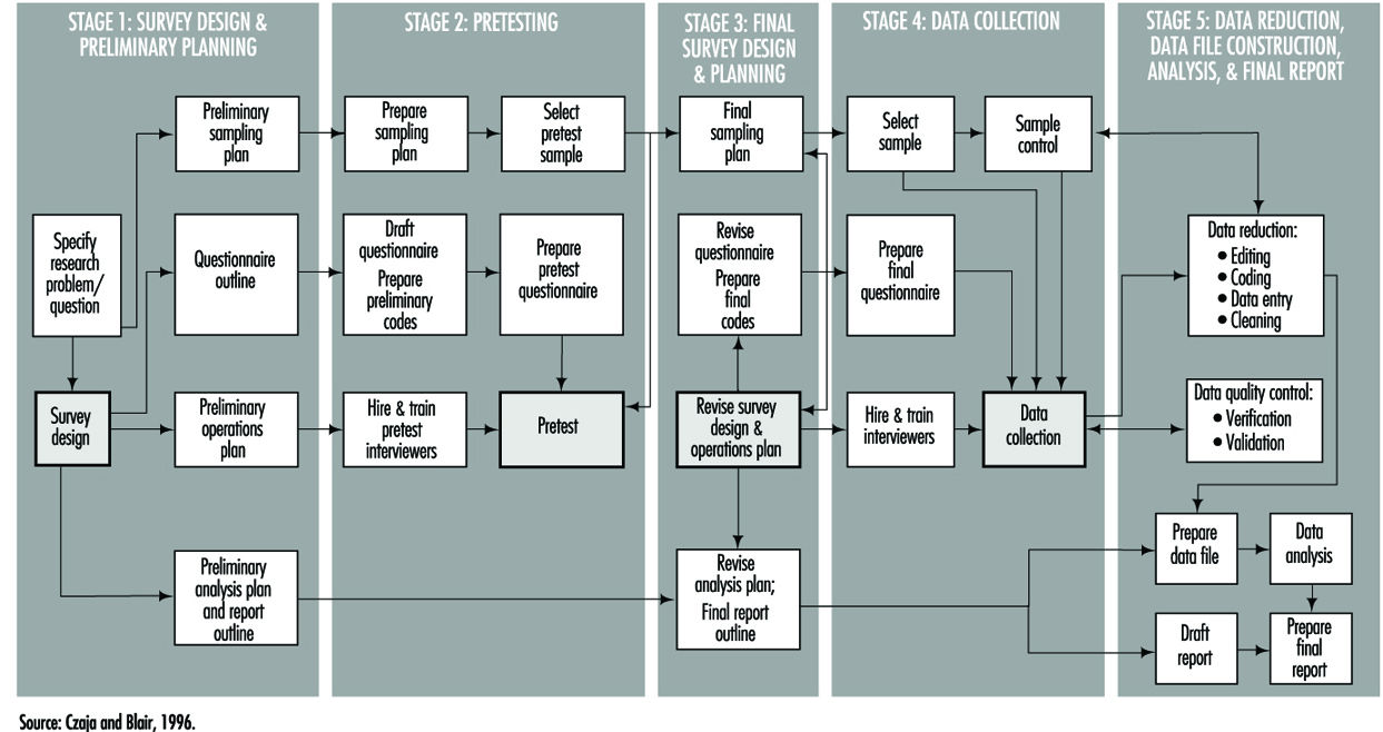
Types of studies and questionnaires

The research goals of the study itself determine the structure, length and content of the questionnaire. These questionnaire attributes are invariably tempered by the method of data collection, which usually falls within one of three modes: in person, mail and telephone. Each of these has its advantages and disadvantages which can affect not only the quality of the data but the validity of the overall study.

A mailed questionnaire is the least expensive format and can cover workers in a wide geographical area. However, in that overall response rates are often low (typically 45 to 75%), it cannot be overly complex since there is little or no opportunity for clarification of questions, and it may be difficult to ascertain whether potential responses to critical exposure or other questions differ systematically between respondents and non-respondents. The physical layout and language must accommodate the least educated of potential study participants, and must be capable of completion in a fairly short time period, typically 20 to 30 minutes.

Telephone questionnaires can be used in population-based studies—that is, surveys in which a sample of a geographically defined population is canvassed—and are a practical method to update information in existing data files. They may be longer and more complex than mailed questionnaires in language and content, and since they are administered by trained interviewers the greater cost of a telephone survey can be partially offset by physically structuring the questionnaire for efficient administration (such as through skip patterns). Response rates are usually better than with mailed questionnaires, but are subject to biases related to increasing use of telephone answering machines, refusals, non-contacts and problems of populations with limited telephone service. Such biases generally relate to the sampling design itself and not especially to the questionnaire. Although telephone questionnaires have long been in use in North America, their feasibility in other parts of the world has yet to be established.

Face-to-face interviews provide the greatest opportunity for collecting accurate complex data; they are also the most expensive to administer, since they require both training and travel for professional staff. The physical layout and order of questions may be arranged to optimize administration time. Studies which utilize in-person interviewing generally have the highest response rates and are subject to the least response bias. This is also the type of interview in which the interviewer is most likely to learn whether or not the participant is a case (in a case-control study) or the participant’s exposure status (in a cohort study). Care must therefore be taken to preserve the objectivity of the interviewer by training him or her to avoid leading questions and body language that might evoke biased responses.

It is becoming more common to use a hybrid study design in which complex exposure situations are assessed in a personal or telephone interview which allows maximum probing and clarification, followed by a mailed questionnaire to capture lifestyle data like smoking and diet.

Confidentiality and research participant issues

Since the purpose of a questionnaire is to obtain data about individuals, questionnaire design must be guided by established standards for ethical treatment of human subjects. These guidelines apply to acquisition of questionnaire data just as they do for biological samples such as blood and urine, or to genetic testing. In the United States and many other countries, no studies involving humans may be conducted with public funds unless approval of questionnaire language and content is first obtained from an appropriate Institutional Review Board. Such approval is intended to assure that questions are confined to legitimate study purposes, and that they do not violate the rights of study participants to answer questions voluntarily. Participants must be assured that their participation in the study is entirely voluntary, and that refusal to answer questions or even to participate at all will not subject them to any penalties or alter their relationship with their employer or medical practitioner.

Participants must also be assured that the information they provide will be held in strict confidence by the investigator, who must of course take steps to maintain the physical security and inviolability of the data. This often entails physical separation of information regarding the identity of participants from computerized data files. It is common practice to advise study participants that their replies to questionnaire items will be used only in aggregation with responses of other participants in statistical reports, and will not be disclosed to the employer, physician or other parties.

Measurement aspects of questionnaire design

One of the most important functions of a questionnaire is to obtain data about some aspect or attribute of a person in either qualitative or quantitative form. Some items may be as simple as weight, height or age, while others may be considerably more complicated, as with an individual’s response to stress. Qualitative responses, such as gender, will ordinarily be converted into numerical variables. All such measures may be characterized by their validity and their reliability. Validity is the degree to which a questionnaire-derived number approaches its true, but possibly unknown, value. Reliability measures the likelihood that a given measurement will yield the same result on repetition, whether that result is close to the “truth” or not. Figure 2 shows how these concepts are related. It demonstrates that a measurement can be valid but not reliable, reliable but not valid, or both valid and reliable.

Figure 2. Validity & reliability relationship

Over the years, many questionnaires have been developed by researchers in order to answer research questions of wide interest. Examples include the Scholastic Aptitude Test, which measures a student’s potential for future academic achievement, and the Minnesota Multiphasic Personality Inventory (MMPI), which measures certain psychosocial characteristics. A variety of other psychological indicators are discussed in the chapter on psychometrics. There are also established physiological scales, such as the British Medical Research Council (BMRC) questionnaire for pulmonary function. These instruments have a number of important advantages. Chief among these are the facts that they have already been developed and tested, usually in many populations, and that their reliability and validity are known. Anyone constructing a questionnaire is well advised to utilize such scales if they fit the study purpose. Not only do they save the effort of “re-inventing the wheel”, but they make it more likely that study results will be accepted as valid by the research community. It also makes for more valid comparisons of results from different studies provided they have been properly used.

The preceding scales are examples of two important types of measures which are commonly used in questionnaires to quantify concepts that may not be fully objectively measurable in the way that height and weight are, or which require many similar questions to fully “tap the domain” of one specific behavioural pattern. More generally, indexes and scales are two data reduction techniques that provide a numerical summary of groups of questions. The above examples illustrate physiological and psychological indexes, and they are also frequently used to measure knowledge, attitude and behaviour. Briefly, an index is usually constructed as a score obtained by counting, among a group of related questions, the number of items that apply to a study participant. For instance, if a questionnaire presents a list of diseases, a disease history index could be the total number of those which a respondent says he or she has had. A scale is a composite measure based on the intensity with which a participant answers one or more related questions. For example, the Likert scale, which is frequently used in social research, is typically constructed from statements with which one may agree strongly, agree weakly, offer no opinion, disagree weakly, or disagree strongly, the response being scored as a number from 1 to 5. Scales and indexes may be summed or otherwise combined to form a fairly complex picture of study participants’ physical, psychological, social or behavioural characteristics.

Validity merits special consideration because of its reflection of the “truth”. Three important types of validity often discussed are face, content and criterion validity. Face validity is a subjective quality of an indicator which insures that the wording of a question is clear and unambiguous. Content validity insures that the questions will serve to tap that dimension of response in which the researcher is interested. Criterion (or predictive) validity is derived from an objective assessment of how closely a questionnaire measurement approaches a separately measurable quantity, as for instance how well a questionnaire assessment of dietary vitamin A intake matches the actual consumption of vitamin A, based upon food consumption as documented with dietary records.

Questionnaire content, quality and length

Wording. The wording of questions is both an art and a professional skill. Therefore, only the most general of guidelines can be presented. It is generally agreed that questions should be devised which:

motivate the participant to respond
draw upon the participant’s personal knowledge
take into account his or her limitations and personal frame of reference, so that the aim and meaning of the questions is easily understood and
elicit a response based upon the participant’s own knowledge and do not require guessing, except possibly for attitude and opinion questions.

Question sequence and structure. Both the order and presentation of questions can affect the quality of information gathered. A typical questionnaire, whether self-administered or read by an interviewer, contains a prologue which introduces the study and its topic to the respondent, provides any additional information he or she will need, and tries to motivate the respondent to answer the questions. Most questionnaires contain a section designed to collect demographic information, such as age, gender, ethnic background and other variables about the participant’s background, including possibly confounding variables. The main subject matter of data collection, such as nature of the workplace and exposure to specific substances, is usually a distinct questionnaire section, and is often preceded by an introductory prologue of its own which might first remind the participant of specific aspects of the job or workplace in order to create a context for detailed questions. The layout of questions that are intended to establish worklife chronologies should be arranged so as to minimize the risk of chronological omissions. Finally, it is customary to thank the respondent for his or her participation.

Types of questions. The designer must decide whether to use open-ended questions in which participants compose their own answers, or closed questions that require a definite response or a choice from a short menu of possible responses. Closed questions have the advantage that they clarify alternatives for the respondent, avoid snap responses, and minimize lengthy rambling that may be impossible to interpret. However, they require that the designer anticipate the range of potential responses in order to avoid losing information, particularly for unexpected situations that occur in many workplaces. This in turn requires well planned pilot testing. The investigator must decide whether and to what extent to permit a “don’t know” response category.

Length. Determining the final length of a questionnaire requires striking a balance between the desire to obtain as much detailed information as possible to achieve the study goals with the fact that if a questionnaire is too lengthy, at some point many respondents will lose interest and either stop responding or respond hastily, inaccurately and without thought in order to bring the session to an end. On the other hand, a questionnaire which is very short may obtain a high response rate but not achieve the study goals. Since respondent motivation often depends on having a personal stake in the outcome, such as improving working conditions, tolerance for a lengthy questionnaire may vary widely, especially when some participants (such as workers in a particular plant) may perceive their stake to be higher than others (such as persons contacted via random telephone dialling). This balance can be achieved only through pilot testing and experience. Interviewer-administered questionnaires should record the beginning and ending time to permit calculation of the duration of the interview. This information is useful in assessing the level of quality of the data.

Language. It is essential to use the language of the population to make the questions understood by all. This may require becoming familiar with local vernacular that may vary within any one country. Even in countries where the same language is nominally spoken, such as Britain and the United States, or the Spanish-speaking countries of Latin America, local idioms and usage may vary in a way that can obscure interpretation. For example, in the US “tea” is merely a beverage, whereas in Britain it may mean “a pot of tea,” “high tea,” or “the main evening meal,” depending on locale and context. It is especially important to avoid scientific jargon, except where study participants can be expected to possess specific technical knowledge.

Clarity and leading questions. While it is often the case that shorter questions are clearer, there are exceptions, especially where a complex subject needs to be introduced. Nevertheless, short questions clarify thinking and reduce unnecessary words. They also reduce the chance of overloading the respondent with too much information to digest. If the purpose of the study is to obtain objective information about the participant’s working situation, it is important to word questions in a neutral way and to avoid “leading” questions that may favour a particular answer, such as “Do you agree that your workplace conditions are harmful to your health?”

Questionnaire layout. The physical layout of a questionnaire can affect the cost and efficiency of a study. It is more important for self-administered questionnaires than those which are conducted by interviewers. A questionnaire which is designed to be completed by the respondent but which is overly complex or difficult to read may be filled out casually or even discarded. Even questionnaires which are designed to be read aloud by trained interviewers need to be printed in clear, readable type, and patterns of question skipping must be indicated in a manner which maintains a steady flow of questioning and minimizes page turning and searching for the next applicable question.

Validity Concerns

Bias

The enemy of objective data gathering is bias, which results from systematic but unplanned differences between groups of people: cases and controls in a case-control study or exposed and non-exposed in a cohort study. Information bias may be introduced when two groups of participants understand or respond differently to the same question. This may occur, for instance, if questions are posed in such a way as to require special technical knowledge of a workplace or its exposures that would be understood by exposed workers but not necessarily by the general public from which controls are drawn.

The use of surrogates for ill or deceased workers has the potential for bias because next-of-kin are likely to recall information in different ways and with less accuracy than the worker himself or herself. The introduction of such bias is especially likely in studies in which some interviews are carried out directly with study participants while other interviews are carried out with relatives or co-workers of other research participants. In either situation, care must be taken to reduce any effect that might arise from the interviewer’s knowledge of the disease or exposure status of the worker of interest. Since it is not always possible to keep interviewers “blind,” it is important to emphasize objectivity and avoidance of leading or suggestive questions or unconscious body language during training, and to monitor performance while the study is being carried out.

Recall bias results when cases and controls “remember” exposures or work situations differently. Hospitalized cases with a potential occupationally related illness may be more capable of recalling details of their medical history or occupational exposures than persons contacted randomly on the telephone. A type of this bias that is becoming more common has been labelled social desirability bias. It describes the tendency of many people to understate, whether consciously or not, their indulgence in “bad habits” such as cigarette smoking or consumption of foods high in fat and cholesterol, and to overstate “good habits” like exercise.

Response bias denotes a situation in which one group of study participants, such as workers with a particular occupational exposure, may be more likely to complete questionnaires or otherwise participate in a study than unexposed persons. Such a situation may result in a biased estimation of the association between exposure and disease. Response bias may be suspected if response rates or the time taken to complete a questionnaire or interview differ substantially between groups (e.g., cases vs. controls, exposed vs. unexposed). Response bias generally differs depending upon the mode of questionnaire administration. Questionnaires which are mailed are usually more likely to be returned by individuals who see a personal stake in study findings, and are more likely to be ignored or discarded by persons selected at random from the general population. Many investigators who utilize mail surveys also build in a follow-up mechanism which may include second and third mailings as well as subsequent telephone contacts with non-respondents in order to maximize response rates.

Studies which utilize telephone surveys, including those which make use of random digit dialling to identify controls, usually have a set of rules or a protocol defining how many times attempts to contact potential respondents must be made, including time of day, and whether evening or weekend calls should be attempted. Those who conduct hospital-based studies usually record the number of patients who refuse to participate, and reasons for non-participation. In all such cases, various measures of response rates are recorded in order to provide an assessment of the extent to which the target population has actually been reached.

Selection bias results when one group of participants preferentially responds or otherwise participates in a study, and can result in biased estimation of the relationship between exposure and disease. In order to assess selection bias and whether it leads to under- or over-estimation of exposure, demographic information such as educational level can be used to compare respondents with non-respondents. For example, if participants with little education have lower response rates than participants with higher education, and if a particular occupation or smoking habit is known to be more frequent in less educated groups, then selection bias with underestimation of exposure for that occupation or smoking category is likely to have occurred.

Confounding is an important type of selection bias which results when the selection of respondents (cases and controls in a case-control study, or exposed and unexposed in a cohort study) depends in some way upon a third variable, sometimes in a manner unknown to the investigator. If not identified and controlled, it can lead unpredictably to underestimates or overestimates of disease risks associated with occupational exposures. Confounding is usually dealt with either by manipulating the design of the study itself (e.g., through matching cases to controls on age and other variables) or at the analysis stage. Details of these techniques are presented in other articles within this chapter.

Documentation

In any research study, all study procedures must be thoroughly documented so that all staff, including interviewers, supervisory personnel and researchers, are clear about their respective duties. In most questionnaire-based studies, a coding manual is prepared which describes on a question-by-question basis everything the interviewer needs to know beyond the literal wording of the questions. This includes instructions for coding categorical responses and may contain explicit instructions on probing, listing those questions for which it is permitted and those for which it is not. In many studies new, unforeseen response choices for certain questions are occasionally encountered in the field; these must be recorded in the master codebook and copies of additions, changes or new instructions distributed to all interviewers in a timely fashion.

Planning, testing and revision

As can be seen from figure 1, questionnaire development requires a great deal of thoughtful planning. Every questionnaire needs to be tested at several stages in order to make certain that the questions “work”, i.e., that they are understandable and produce responses of the intended quality. It is useful to test new questions on volunteers and then to interrogate them at length to determine how well specific questions were understood and what types of problems or ambiguities were encountered. The results can then be utilized to revise the questionnaire, and the procedure can be repeated if necessary. The volunteers are sometimes referred to as a “focus group”.

All epidemiological studies require pilot testing, not only for the questionnaires, but for the study procedures as well. A well designed questionnaire serves its purpose only if it can be delivered efficiently to the study participants, and this can be determined only by testing procedures in the field and making adjustments when necessary.

Interviewer training and supervision

In studies which are conducted by telephone or face-to-face interview, the interviewer plays a critical role. This person is responsible not simply for presenting questions to the study participants and recording their responses, but also for interpreting those responses. Even with the most rigidly structured interview study, respondents occasionally request clarification of questions, or offer responses which do not fit the available response categories. In such cases the interviewer’s job is to interpret either the question or the response in a manner consistent with the intent of the researcher. To do so effectively and consistently requires training and supervision by an experienced researcher or manager. When more than one interviewer is employed on a study, interviewer training is especially important to insure that questions are presented and responses interpreted in a uniform manner. In many research projects this is accomplished in group training settings, and is repeated periodically (e.g., annually) in order to keep the interviewers’ skills fresh. Training seminars commonly cover the following topics in considerable detail:

general introduction to the study
informed consent and confidentiality issues
how to introduce the interview and how to interact with respondents
the intended meaning of each question
instructions for probing, i.e., offering the respondent further opportunity to clarify or embellish responses
discussion of typical problems which arise during interviews.

Study supervision often entails onsite observation, which may include tape-recording of interviews for subsequent dissection. It is common practice for the supervisor to personally review every questionnaire prior to approving and submitting it to data entry. The supervisor also sets and enforces performance standards for interviewers and in some studies conducts independent re-interviews with selected participants as a reliability check.

Data collection

The actual distribution of questionnaires to study participants and subsequent collection for analysis is carried out using one of the three modes described above: by mail, telephone or in person. Some researchers organize and even perform this function themselves within their own institutions. While there is considerable merit to a senior investigator becoming familiar with the dynamics of the interview at first hand, it is most cost effective and conducive to maintaining high data quality for trained and well-supervised professional interviewers to be included as part of the research team.

Some researchers make contractual arrangements with companies that specialize in survey research. Contractors can provide a range of services which may include one or more of the following tasks: distributing and collecting questionnaires, carrying out telephone or face-to-face interviews, obtaining biological specimens such as blood or urine, data management, and statistical analysis and report writing. Irrespective of the level of support, contractors are usually responsible for providing information about response rates and data quality. Nevertheless, it is the researcher who bears final responsibility for the scientific integrity of the study.

Reliability and re-interviews

Data quality may be assessed by re-interviewing a sample of the original study participants. This provides a means for determining the reliability of the initial interviews, and an estimate of the repeatability of responses. The entire questionnaire need not be re-administered; a subset of questions usually is sufficient. Statistical tests are available for assessing the reliability of a set of questions asked of the same participant at different times, as well as for assessing the reliability of responses provided by different participants and even for those queried by different interviewers (i.e., inter- and intra-rater assessments).

Technology of questionnaire processing

Advances in computer technology have created many different ways in which questionnaire data can be captured and made available to the researcher for computer analysis. There are three fundamentally different ways in which data can be computerized: in real time (i.e., as the participant responds during an interview), by traditional key entry methods, and by optical data capture methods.

Computer-aided data capture

Many researchers now use computers to collect responses to questions posed in both face-to-face and telephone interviews. Researchers in the field find it convenient to use laptop computers which have been programmed to display the questions sequentially and which permit the interviewer to enter the response immediately. Survey research companies which do telephone interviewing have developed analogous systems called computer-aided telephone interview (CATI) systems. These methods have two important advantages over more traditional paper questionnaires. First, responses can be instantly checked against a range of permissible answers and for consistency with previous responses, and discrepancies can be immediately brought to the attention of both the interviewer and the respondent. This greatly reduces the error rate. Secondly, skip patterns can be programmed to minimize administration time.

The most common method for computerizing data still is the traditional key entry by a trained operator. For very large studies, questionnaires are usually sent to a professional contract company which specializes in data capture. These firms often utilize specialized equipment which permits one operator to key a questionnaire (a procedure sometimes called keypunch for historical reasons) and a second operator to re-key the same data, a process called key verification. Results of the second keying are compared with the first to assure the data have been entered correctly. Quality assurance procedures can be programmed which ensure that each response falls within an allowable range, and that it is consistent with other responses. The resulting data files can be transmitted to the researcher on disk, tape or electronically by telephone or other computer network.

For smaller studies, there are numerous commercial PC-based programs which have data entry features which emulate those of more specialized systems. These include database programs such as dBase, Foxpro and Microsoft Access, as well as spreadsheets such as Microsoft Excel and Lotus 1-2-3. In addition, data entry features are included with many computer program packages whose principal purpose is statistical data analysis, such as SPSS, BMDP and EPI INFO.

One widespread method of data capture which works well for certain specialized questionnaires uses optical systems. Optical mark reading or optical sensing is used to read responses on questionnaires that are specially designed for participants to enter data by marking small rectangles or circles (sometimes called “bubble codes”). These work most efficiently when each individual completes his or her own questionnaire. More sophisticated and expensive equipment can read hand-printed characters, but at present this is not an efficient technique for capturing data in large-scale studies.

Archiving Questionnaires and Coding Manuals

Because information is a valuable resource and is subject to interpretation and other influences, researchers sometimes are asked to share their data with other researchers. The request to share data can be motivated by a variety of reasons, which may range from a sincere interest in replicating a report to concern that data may not have been analysed or interpreted correctly.

Where falsification or fabrication of data is suspected or alleged, it becomes essential that the original records upon which reported findings are based be available for audit purposes. In addition to the original questionnaires and/or computer files of raw data, the researcher must be able to provide for review the coding manual(s) developed for the study and the log(s) of all data changes which were made in the course of data coding, computerization and analysis. For example, if a data value had been altered because it had initially appeared as an outlier, then a record of the change and the reasons for making the change should have been recorded in the log for possible data audit purposes. Such information also is of value at the time of report preparation because it serves as a reminder about how the data which gave rise to the reported findings had actually been handled.

For these reasons, upon completion of a study, the researcher has an obligation to ensure that all basic data are appropriately archived for a reasonable period of time, and that they could be retrieved if the researcher were called upon to provide them.

Back

Published in 28. Epidemiology and Statistics

Monday, 07 March 2011 18:13

Asbestos: Historical Perspective

Several examples of workplace hazards often are quoted to exemplify not only the possible adverse health effects associated with workplace exposures, but also to reveal how a systematic approach to the study of worker populations can uncover important exposure-disease relationships. One such example is that of asbestos. The simple elegance with which the late Dr. Irving J. Selikoff demonstrated the elevated cancer risk among asbestos workers has been documented in an article by Lawrence Garfinkel. It is reprinted here with only slight modification and with the permission of CA-A Cancer Journal for Clinicians (Garfinkel 1984). The tables came from the original article by Dr. Selikoff and co-workers (1964).

Asbestos exposure has become a public health problem of considerable magnitude, with ramifications that extend beyond the immediate field of health professionals to areas served by legislators, judges, lawyers, educators, and other concerned community leaders. As a result, asbestos-related diseases are of increasing concern to clinicians and health authorities, as well as to consumers and the public at large.

Historical Background

Asbestos is a highly useful mineral that has been utilized in diverse ways for many centuries. Archaeological studies in Finland have shown evidence of asbestos fibres incorporated in pottery as far back as 2500 BC. In the 5th century BC, it was used as a wick for lamps. Herodotus commented on the use of asbestos cloth for cremation about 456 BC. Asbestos was used in body armour in the 15th century, and in the manufacture of textiles, gloves, socksand handbags in Russia c. 1720. Although it is uncertain when the art of weaving asbestos was developed, we know that the ancients often wove asbestos with linen. Commercial asbestos production began in Italy about 1850, in the making of paper and cloth.

The development of asbestos mining in Canada and South Africa about 1880 reduced costs and spurred the manufacture of asbestos products. Mining and production of asbestos in the United States, Italy and Russia followed soon after. In the United States, the development of asbestos as pipe insulation increased production and was followed shortly thereafter by other varied uses including brake linings, cement pipes, protective clothing and so forth.

Production in the US increased from about 6,000 tons in 1900 to 650,000 tons in 1975, although by 1982, it was about 300,000 tons and by 1994, production had dropped to 33,000 tons.

It is reported that Pliny the Younger (61-113 AD) commented on the sickness of slaves who worked with asbestos. Reference to occupational disease associated with mining appeared in the 16th century, but it was not until 1906 in England that the first reference to pulmonary fibrosis in an asbestos worker appeared. Excess deaths in workers involved with asbestos manufacturing applications were reported shortly thereafter in France and Italy, but major recognition of asbestos-induced disease began in England in 1924. By 1930, Wood and Gloyne had reported on 37 cases of pulmonary fibrosis.

The first reference to carcinoma of the lung in a patient with “asbestos-silicosis” appeared in 1935. Several other case reports followed. Reports of high percentages of lung cancer in patients who died of asbestosis appeared in 1947, 1949 and 1951. In 1955 Richard Doll in England reported an excess risk of lung cancer in persons who had worked in an asbestos plant since 1935, with an especially high risk in those who were employed more than 20 years.

Clinical Observations

It was against this background that Dr. Irving Selikoff’s clinical observations of asbestos-related disease began. Dr. Selikoff was at that time already a distinguished scientist. His prior accomplishments included the development and first use of isoniazid in the treatment of tuberculosis, for which he received a Lasker Award in 1952.

In the early 1960s, as a chest physician practising in Paterson, New Jersey, he had observed many cases of lung cancer among workers in an asbestos factory in the area. He decided to extend his observations to include two locals of the asbestos insulator workers union, whose members also had been exposed to asbestos fibres. He recognized that there were still many people who did not believe that lung cancer was related to asbestos exposure and that only a thorough study of a total exposed population could convince them. There was the possibility that asbestos exposure in the population could be related to other types of cancer, such as pleural and peritoneal mesothelioma, as had been suggested in some studies, and perhaps other sites as well. Most of the studies of the health effects of asbestos in the past had been concerned with workers exposed in the mining and production of asbestos. It was important to know if asbestos inhalation also affected other asbestos-exposed groups.

Dr. Selikoff had heard of the accomplishments of Dr. E. Cuyler Hammond, then Director of the Statistical Research Section of the American Cancer Society (ACS), and decided to ask him to collaborate in the design and analysis of a study. It was Dr. Hammond who had written the landmark prospective study on smoking and health published a few years earlier.

Dr. Hammond immediately saw the potential importance of a study of asbestos workers. Although he was busily engaged in analysing data from the then new ACS prospective study, Cancer Prevention Study I (CPS I), which he had begun a few years earlier, he readily agreed to a collaboration in his “spare time”. He suggested confining the analysis to those workers with at least 20 years’ work experience, who thus would have had the greatest amount of asbestos exposure.

The team was joined by Mrs. Janet Kaffenburgh, a research associate of Dr. Selikoff’s at Mount Sinai Hospital, who worked with Dr. Hammond in preparing the lists of the men in the study, including their ages and dates of employment and obtaining the data on facts of death and causes from union headquarters records. This information was subsequently transferred to file cards that were sorted literally on the living room floor of Dr. Hammond’s house by Dr. Hammond and Mrs. Kaffenburgh.

Dr. Jacob Churg, a pathologist at Barnert Memorial Hospital Center in Paterson, New Jersey, provided pathologic verification of the cause of death.

Tabe 1. Man-years of experience of 632 asbestos workers exposed to asbestos dust 20 years or longer

Age		Time period
	1943-47	1948-52	1953-57	1958-62
35–39	85.0	185.0	7.0	11.0
40–44	230.5	486.5	291.5	70.0
45–49	339.5	324.0	530.0	314.5
50–54	391.5	364.0	308.0	502.5
55–59	382.0	390.0	316.0	268.5
60–64	221.0	341.5	344.0	255.0
65–69	139.0	181.0	286.0	280.0
70–74	83.0	115.5	137.0	197.5
75–79	31.5	70.0	70.5	75.0
80–84	5.5	18.5	38.5	23.5
85+	3.5	2.0	8.0	13.5
Total	1,912.0	2,478.0	2,336.5	2,011.0

The resulting study was of the type classified as a “prospective study retrospectively carried out”. The nature of the union records made it possible to accomplish an analysis of a long-range study in a relatively short period of time. Although only 632 men were involved in the study, there were 8,737 man-years of exposure to risk (see table 1); 255 deaths occurred during the 20-year period of observation from 1943 through 1962 (see table 2). It is in table 28.17 where the observed number of deaths can be seen invariably to exceed the number expected, demonstrating the association between workplace asbestos exposure and an elevated cancer death rate.

Table 2. Observed and expected number of deaths among 632 asbestos workers exposed to asbestos dust 20 years or longer

Cause of death	Time period				Total
	1943-47	1948-52	1953-57	1958-62	1943-62
Total, all causes
Observed (asbestos workers)	28.0	54.0	85.0	88.0	255.0
Expected (US White males)	39.7	50.8	56.6	54.4	203.5
Total cancer, all sites
Observed (asbestos workers)	13.0	17.0	26.0	39.0	95.0
Expected (US White males)	5.7	8.1	13.0	9.7	36.5
Cancer of lung and pleura
Observed (asbestos workers)	6.0	8.0	13.0	18.0	45.0
Expected (US White males)	0.8	1.4	2.0	2.4	6.6
Cancer of stomach, colon and rectum
Observed (asbestos workers)	4.0	4.0	7.0	14.0	29.0
Expected (US White males)	2.0	2.5	2.6	2.3	9.4
Cancer of all other sites combined
Observed (asbestos workers)	3.0	5.0	6.0	7.0	21.0
Expected (US White males)	2.9	4.2	8.4	5.0	20.5

Significance of the Work

This paper constituted a turning point in our knowledge of asbestos-related disease and set the direction of future research. The article has been cited in scientific publications at least 261 times since it was originally published. With financial support from the ACS and the National Institutes of Health, Dr. Selikoff and Dr. Hammond and their growing team of mineralogists, chest physicians, radiologists, pathologists, hygienists and epidemiologists continued to explore various facets of asbestos disease.

A major paper in 1968 reported the synergistic effect of cigarette smoking on asbestos exposure (Selikoff, Hammond and Churg 1968). The studies were expanded to include asbestos production workers, persons indirectly exposed to asbestos in their work (shipyard workers, for example) and those with family exposure to asbestos.

In a later analysis, in which the team was joined by Herbert Seidman, MBA, Assistant Vice President for Epidemiology and Statistics of the American Cancer Society, the group demonstrated that even short-term exposure to asbestos resulted in a significant increased risk of cancer up to 30 years later (Seidman, Selikoff and Hammond 1979). There were only three cases of mesothelioma in this first study of 632 insulators, but later investigations showed that 8% of all deaths among asbestos workers were due to pleural and peritoneal mesothelioma.

As Dr. Selikoff’s scientific investigations expanded, he and his co-workers made noteworthy contributions toward reducing exposure to asbestos through innovations in industrial hygiene techniques; by persuading legislators about the urgency of the asbestos problem; in evaluating the problems of disability payments in connection with asbestos disease; and in investigating the general distribution of asbestos particles in water supplies and in the ambient air.

Dr. Selikoff also called the medical and scientific community’s attention to the asbestos problem by organizing conferences on the subject and participating in many scientific meetings. Many of his orientation meetings on the problem of asbestos disease were structured particularly for lawyers, judges, presidents of large corporations and insurance executives.

Back

Published in 28. Epidemiology and Statistics

" DISCLAIMER: The ILO does not take responsibility for content presented on this web portal that is presented in any language other than English, which is the language used for the initial production and peer-review of original content. Certain statistics have not been updated since the production of the 4th edition of the Encyclopaedia (1998)."

Table of Contents

Tables and Figures

Tables

Figures

Epidemiological Method Applied to Occupational Health and Safety

Exposure Assessment

Summary Worklife Exposure Measures

Measuring Effects of Exposures

Options in Study Design

Validity Issues in Study Design

Impact of Random Measurement Error

Statistical Methods

Causality Assessment and Ethics in Epidemiological Research

Case Studies Illustrating Methodological Issues in the Surveillance of Occupational Diseases

More...

Questionnaires in Epidemiological Research

Asbestos: Historical Perspective

Contents