k2 Feed

Monday, 28 February 2011 21:34

Diseases Caused by Organic Dusts

Organic Dust and Disease

Dusts of vegetable, animal and microbial origin have always been part of the human environment. When the first aquatic organisms moved to land some 450 million years ago, they soon developed defence systems against the many noxious substances present in the terrestrial environment, most of them of plant origin. Exposures to this environment usually cause no specific problems, even though plants contain a number of extremely toxic substances, particularly those present in or produced by moulds.

During the development of civilization, climatic conditions in some parts of the world necessitated certain activities to be undertaken indoors. Threshing in the Scandinavian countries was performed indoors during the winter, a practice mentioned by chroniclers in antiquity. The enclosure of dusty processes led to disease among the exposed persons, and one of the first published accounts of this is by the Danish bishop Olaus Magnus (1555, as cited by Rask-Andersen 1988). He described a disease among threshers in Scandinavia as follows:

“In separating the grain from the chaff, care must be taken to choose a time when there is a suitable wind which will sweep away the grain dust, so that it will not damage the vital organs of the threshers. This dust is so fine that it will almost unnoticeably penetrate into the mouth and accumulate in the throat. If this is not quickly dealt with by drinking fresh ale, the thresher may never again or only for a short period eat what he has threshed.”

With the introduction of machine processing of organic materials, treatment of large quantities of materials indoors with poor ventilation led to high levels of airborne dust. The descriptions by bishop Olaus Magnus and later by Ramazzini (1713) were followed by several reports on disease and organic dusts in the nineteenth century, particularly among cotton mill workers (Leach 1863; Prausnitz 1936). Later, the specific pulmonary disease common among farmers handling mouldy materials was also described (Campbell 1932).

During recent decades, a large number of reports on disease among persons exposed to organic dusts have been published. Initially, most of these were based on persons seeking medical help. The names of the diseases, when published, were often related to the particular environment where the disease was first recognized, and a bewildering array of names resulted, such as farmer’s lung, mushroom grower’s lung, brown lung and humidifier fever.

With the advent of modern epidemiology, more reliable figures were obtained for the incidence of occupational respiratory diseases related to organic dust (Rylander, Donham and Peterson 1986; Rylander and Peterson 1990). There was also advancement in the understanding of the pathological mechanisms underlying these diseases, particularly the inflammatory response (Henson and Murphy 1989). This paved the way for a more coherent picture of diseases caused by organic dusts (Rylander and Jacobs 1997).

The following will describe the different organic dust environments where disease has been reported, the disease entities themselves, the classical byssinosis disease and specific preventive measures.

Environments

Organic dusts are airborne particles of vegetable, animal or microbial origin. Table 1 lists examples of environments, work processes and agents involving the risk of exposure to organic dusts.

Table 1. Examples of sources of hazards of exposure to organic dust

Agriculture

Handling of grain, hay or other crops

Sugar-cane processing

Greenhouses

Silos

Animals

Swine/dairy confinement buildings

Poultry houses and processing plants

Laboratory animals, farm animals and pets

Waste-processing

Sewage water and silt

Household garbage

Composting

Industry

Vegetable fibre processing (cotton, flax, hemp, jute, sisal)

Fermentation

Timber and wood processing

Bakeries

Biotechnology processing

Buildings

Contaminated water in humidifiers

Microbial growth on structures or in ventilation ducts

Agents

It is now understood that the specific agents in the dusts are the major reason why disease develops. Organic dusts contain a multitude of agents with potential biological effects. Some of the major agents are found in table 2.

Table 2. Major agents in organic dusts with potential biological activity

Vegetable agents

Tannins

Histamine

Plicatic acid

Alkaloids (e.g., nicotine)

Cytochalasins

Animal agents

Proteins

Enzymes

Microbial agents

Endotoxins

(1→3)–β–D-glucans

Proteases

Mycotoxins

The relative role of each of these agents, alone or in combination with others, for the development of disease, is mostly unknown. Most of the information available relates to bacterial endotoxins which are present in all organic dusts.

Endotoxins are lipopolysaccharide compounds which are attached to the outer cell surface of Gram-negative bacteria. Endotoxin has a wide variety of biological properties. After inhalation it causes an acute inflammation (Snella and Rylander 1982; Brigham and Meyrick 1986). An influx of neutrophils (leukocytes) into the lung and the airways is the hallmark of this reaction. It is accompanied by activation of other cells and secretion of inflammatory mediators. After repeated exposures, the inflammation decreases (adaptation). The reaction is limited to the airway mucosa, and there is no extensive involvement of the lung parenchyma.

Another specific agent in organic dust is (1→3)-β-D-glucan. This is a polyglucose compound present in the cell wall structure of moulds and some bacteria. It enhances the inflammatory response caused by endotoxin and alters the function of inflammatory cells, particularly macrophages and T-cells (Di Luzio 1985; Fogelmark et al. 1992).

Other specific agents present in organic dusts are proteins, tannins, proteases and other enzymes, and toxins from moulds. Very little data are available on the concentrations of these agents in organic dusts. Several of the specific agents in organic dusts, such as proteins and enzymes, are allergens.

Diseases

The diseases caused by organic dusts are shown in table 3 with the corresponding International Classification of Disease (ICD) numbers (Rylander and Jacobs 1994).

Table 3. Diseases induced by organic dusts and their ICD codes

Bronchitis and pneumonitis (ICD J40)

Toxic pneumonitis (inhalation fever, organic dust toxic syndrome)

Airways inflammation (mucous membrane inflammation)

Chronic bronchitis (ICD J42)

Hypersensitivity pneumonitis (allergic alveolitis) (ICD J67)

Asthma (ICD J45)

Rhinitis, conjunctivitis

The primary route of exposure for organic dusts is by inhalation, and consequently the effects on the lung have received the major share of attention in research as well as in clinical work. There is, however, a growing body of evidence from published epidemiological studies and case reports as well as anecdotal reports, that systemic effects also occur. The mechanism involved seems to be a local inflammation at the target site, the lung, and a subsequent release of cytokines either with systemic effects (Dunn 1992; Michel et al. 1991) or an effect on the epithelium in the gut (Axmacher et al. 1991). Non-respiratory clinical effects are fever, joint pains, neurosensory effects, skin problems, intestinal disease, fatigue and headache.

The different disease entities as described in table 3 are easy to diagnose in typical cases, and the underlying pathology is distinctly different. In real life, however, a worker who has a disease due to organic dust exposure, often presents a mixture of the different disease entities. One person may have airways inflammation for a number of years, suddenly develop asthma and in addition have symptoms of toxic pneumonitis during a particularly heavy exposure. Another person may have subclinical hypersensitivity pneumonitis with lymphocytosis in the airways and develop toxic pneumonitis during a particularly heavy exposure.

A good example of the mixture of disease entities that may appear is byssinosis. This disease was first described in the cotton mills, but the individual disease entities are also found in other organic dust environments. An overview of the disease follows.

Byssinosis

The disease

Byssinosis was first described in the 1800s, and a classic report involving clinical as well as experimental work was given by Prausnitz (1936). He described the symptoms among cotton mill workers as follows:

“After working for years without any appreciable trouble except a little cough, cotton mill workers notice either a sudden aggravation of their cough, which becomes dry and exceedingly irritating¼ These attacks usually occur on Mondays ¼ but gradually the symptoms begin to spread over the ensuing days of the week; in time the difference disappears and they suffer continuously.”

The first epidemiological investigations were performed in England in the 1950s (Schilling et al. 1955; Schilling 1956). The initial diagnosis was based on the appearance of a typical Monday morning chest tightness, diagnosed using a questionnaire (Roach and Schilling 1960). A scheme for grading the severity of byssinosis based on the type and periodicity of symptoms was developed (Mekky, Roach and Schilling 1967; Schilling et al. 1955). Duration of exposure was used as a measure of dose and this was related to the severity of the response. Based on clinical interviews of large numbers of workers, this grading scheme was later modified to more accurately reflect the time intervals for the decrease in FEV₁ (Berry et al. 1973).

In one study, a difference in the prevalence of byssinosis in mills processing different types of cotton was found (Jones et al. 1979). Mills using high-quality cotton to produce finer yarns had a lower prevalence of byssinosis than mills producing coarse yarns and using a lower quality of cotton. Thus in addition to exposure intensity and duration, both dose-related variables, the type of dust became an important variable for assessing exposure. Later it was demonstrated that the differences in the response of workers exposed to coarse and medium cottons was dependent not only on the type of cotton but on other variables that affect exposure, including: processing variables such as carding speed, environmental variables such as humidification and ventilation, and manufacturing variables such as different yarn treatments (Berry et al. 1973).

The next refinement of the relationship between exposure to cotton dust and a response (either symptoms or objective measures of pulmonary function), was the studies from the United States, comparing those who worked in 100% cotton to workers using the same cotton but in a 50:50 blend with synthetics and workers without exposure to cotton (Merchant et al. 1973). Workers exposed to 100% cotton had the highest prevalence of byssinosis independent of cigarette smoking, one of the confounders of exposure to cotton dust. This semiquantitative relationship between dose and response to cotton dust was further refined in a group of textile workers stratified by sex, smoking, work area and mill type. A relationship was observed in each of these categories between dust concentration in the lower dust ranges and byssinosis prevalence and/or change in forced expiratory volume in one second (FEV₁).

In later investigations, the FEV₁ decrease over the work shift has been used to assess the effects of exposure, and it is also a part of the US Cotton Dust Standard.

Byssinosis was long regarded as a peculiar disease with a mixture of different symptoms and no knowledge of the specific pathology. Some authors suggested that it was an occupational asthma (Bouhuys 1976). A workgroup meeting in 1987 analysed the symptomatology and pathology of the disease (Rylander et al. 1987). It was agreed that the disease comprised several clinical entities, generally related to organic dust exposure.

Toxic pneumonitis may appear the first time an employee works in the mill, particularly when working in the opening, blowing and carding sections (Trice 1940). Although habituation develops, the symptoms may reappear after an unusually heavy exposure later on.

Airways inflammation is the most widespread disease, and it appears at different degrees of severity from light irritation in the nose and airways to severe dry cough and breathing difficulties. The inflammation causes constriction of airways and a reduced FEV₁. Airway responsiveness is increased as measured with a methacholine or histamine challenge test. It has been discussed whether airways inflammation should be accepted as a disease entity by itself or whether it merely represents a symptom. As the clinical findings in terms of severe cough with airways narrowing can lead to a decrease in work ability, it is justified to regard it as an occupational disease.

Continued airways inflammation over several years may develop into chronic bronchitis, particularly among heavily exposed workers in the blowing and carding areas. The clinical picture would be one of chronic obstructive pulmonary disease (COPD).

Occupational asthma develops in a small percentage of the workforce, but is usually not diagnosed in cross-sectional studies as the workers are forced to leave work because of the disease. Hypersensitivity pneumonitis has not been detected in any of the epidemiological studies undertaken, nor have there been case reports relating to cotton dust exposure. The absence of hypersensitivity pneumonitis may be due to the relatively low amount of moulds in cotton, as mouldy cotton is not acceptable for processing.

A subjective feeling of chest tightness, most common on Mondays, is the classical symptom of cotton dust exposure (Schilling et al. 1955). It is not, however, a feature unique to cotton dust exposure as it appears also among persons working with other kinds of organic dusts (Donham et al. 1989). Chest tightness develops slowly over a number of years but it can also be induced in previously unexposed persons, provided that the dose level is high (Haglind and Rylander 1984). The presence of chest tightness is not directly related to a decrease in FEV₁.

The pathology behind chest tightness has not been explained. It has been suggested that the symptoms are due to an increased adhesiveness of platelets which accumulate in the lung capillaries and increase the pulmonary artery pressure. It is likely that chest tightness involves some kind of cell sensitization, as it takes repeated exposures for the symptom to develop. This hypothesis is supported by results from studies on blood monocytes from cotton workers (Beijer et al. 1990). A higher ability to produce procoagulant factor, indicative of cell sensitization, was found among cotton workers as compared to controls.

The environment

The disease was originally described among workers in cotton, flax and soft hemp mills. In the first phase of cotton treatment within the mills—bale opening, blowing and carding—more than half of the workers may have symptoms of chest tightness and airways inflammation. The incidence decreases as the cotton is processed, reflecting the successive cleaning of the causative agent from the fibre. Byssinosis has been described in all countries where investigations in cotton mills have been performed. Some countries like Australia have, however, unusually low incidence figures (Gun et al. 1983).

There is now uniform evidence that bacterial endotoxins are the causative agent for toxic pneumonitis and airways inflammation (Castellan et al. 1987; Pernis et al. 1961; Rylander, Haglind and Lundholm 1985; Rylander and Haglind 1986; Herbert et al. 1992; Sigsgaard et al. 1992). Dose-response relationships have been described and the typical symptoms have been induced by inhalation of purified endotoxin (Rylander et al. 1989; Michel et al. 1995). Although this does not exclude the possibility that other agents could contribute to the pathogenesis, endotoxins can serve as markers for disease risk. It is unlikely that endotoxins are related to the development of occupational asthma, but they could act as an adjuvant for potential allergens in cotton dust.

The case

The diagnosis of byssinosis is classically made using questionnaires with the specific question “Does your chest feel tight, and if so, on which day of the week?”. Persons with Monday morning chest tightness are classified as byssinotics according to a scheme suggested by Schilling (1956). Spirometry can be performed, and, according to the different combinations of chest tightness and decrease in FEV₁, the diagnostic scheme illustrated in table 4 has evolved.

Table 4. Diagnostic criteria for byssinosis

Grade ½. Chest tightness on the first day of some working weeks

Grade 1. Chest tightness on the first day of every working week

Grade 2. Chest tightness on the first and other days of the working week

Grade 3. Grade 2 symptoms accompanied by evidence of permanent incapacity in the form of diminished effort intolerance and/or reduced ventilatory capacity

Treatment

Treatment in the light stages of byssinosis is symptomatic, and most of the workers learn to live with the slight chest tightness and bronchoconstriction that they experience on Mondays or when cleaning machinery or carrying out similar tasks with a higher than normal exposure. More advanced stages of airways inflammation or regular chest tightness several days of the week require transfer to less dusty operations. The presence of occupational asthma mostly requires work change.

Prevention

Prevention in general is dealt with in detail elsewhere in the Encyclopaedia. The basic principles for prevention in terms of product substitute, exposure limitation, worker protection and screening for disease apply also for cotton dust exposure.

Regarding product substitutes, it has been suggested that cotton with a low level of bacterial contamination be used. An inverse proof of this concept is found in reports from 1863 where the change to dirty cotton provoked an increase in the prevalence of symptoms among the exposed workers (Leach 1863). There is also the possibility of changing to other fibres, particularly synthetic fibres, although this is not always feasible from a product point of view. There is at present no production-applied technique to decrease the endotoxin content of cotton fibres.

Regarding dust reduction, successful programmes have been implemented in the United States and elsewhere (Jacobs 1987). Such programmes are expensive, and the costs for highly efficient dust removal may be prohibitive for developing countries (Corn 1987).

Regarding exposure control, the level of dust is not a sufficiently precise measure of exposure risk. Depending on the degree of contamination with Gram-negative bacteria and thus endotoxin, a given dust level may or may not be associated with a risk. For endotoxins, no official guidelines have been established. It has been suggested that a level of 200 ng/m³ is the threshold for toxic pneumonitis, 100 to 200 ng/m³ for acute airways constriction over the workshift and 10 ng/m³ for airways inflammation (Rylander and Jacobs 1997).

Knowledge about the risk factors and the consequences of exposure are important for prevention. The information basis has expanded rapidly during recent years, but much of it is not yet present in textbooks or other easily available sources. A further problem is that symptoms and findings in respiratory diseases induced by organic dust are non-specific and occur normally in the population. They may thus not be correctly diagnosed in the early stages.

Proper dissemination of knowledge concerning the effects of cotton and other organic dusts requires the establishment of appropriate training programmes. These should be directed not only towards workers with potential exposure but also towards employers and health personnel, particularly occupational health inspectors and engineers. Information must include source identification, symptoms and disease description, and methods of protection. An informed worker can more readily recognize work-related symptoms and communicate more effectively to a health care provider. Regarding health surveillance and screening, questionnaires are a major instrument to be used. Several versions of questionnaires specifically designed for diagnosing diseases induced by organic dust have been reported in the literature (Rylander, Peterson and Donham 1990; Schwartz et al. 1995). Lung function testing is also a useful tool for surveillance and diagnosis. Measurements of airway responsiveness have been found to be useful (Rylander and Bergström 1993; Carvalheiro et al. 1995). Other diagnostic tools such as measurements of inflammatory mediators or cell activity are still in the research phase.

Back

Published in 10. Respiratory System

Monday, 28 February 2011 21:32

Occupational Asthma

Asthma is a respiratory disease characterized by airway obstruction that is partially or completely reversible, either spontaneously or with treatment; airway inflammation; and increased airway responsiveness to a variety of stimuli (NAEP 1991). Occupational asthma (OA) is asthma that is caused by environmental exposures in the workplace. Several hundred agents have been reported to cause OA. Pre-existing asthma or airway hyper-responsiveness, with symptoms worsened by work exposure to irritants or physical stimuli, is usually classified separately as work-aggravated asthma (WAA). There is general agreement that OA has become the most prevalent occupational lung disease in developed countries, although estimates of actual prevalence and incidence are quite variable. It is clear, however, that in many countries asthma of occupational aetiology causes a largely unrecognized burden of disease and disability with high economic and non-economic costs. Much of this public health and economic burden is potentially preventable by identifying and controlling or eliminating the workplace exposures causing the asthma. This article will summarize current approaches to recognition, management and prevention of OA. Several recent publications discuss these issues in more detail (Chan-Yeung 1995; Bernstein et al. 1993).

Magnitude of the Problem

Prevalences of asthma in adults generally range from 3 to 5%, depending on the definition of asthma and geographic variations, and may be considerably higher in some low-income urban populations. The proportion of adult asthma cases in the general population that is related to the work environment is reported to range from 2 to 23%, with recent estimates tending towards the higher end of the range. Prevalences of asthma and OA have been estimated in small cohort and cross-sectional studies of high-risk occupational groups. In a review of 22 selected studies of workplaces with exposures to specific substances, prevalences of asthma or OA, defined in various ways, ranged from 3 to 54%, with 12 studies reporting prevalences over 15% (Becklake, in Bernstein et al. 1993). The wide range reflects real variation in actual prevalence (due to different types and levels of exposure). It also reflects differences in diagnostic criteria, and variation in the strength of the biases, such as “survivor bias” which may result from exclusion of workers who developed OA and left the workplace before the study was conducted. Population estimates of incidence range from 14 per million employed adults per year in the United States to 140 per million employed adults per year in Finland (Meredith and Nordman 1996). Ascertainment of cases was more complete and methods of diagnosis were generally more rigorous in Finland. The evidence from these different sources is consistent in its implication that OA is often under-diagnosed and/or under-reported and is a public health problem of greater magnitude than generally recognized.

Causes of Occupational Asthma

Over 200 agents (specific substances, occupations or industrial processes) have been reported to cause OA, based on epidemiological and/or clinical evidence. In OA, airway inflammation and bronchoconstriction can be caused by immunological response to sensitizing agents, by direct irritant effects, or by other non-immunological mechanisms. Some agents (e.g., organophosphate insecticides) may also cause bronchoconstriction by direct pharmacological action. Most of the reported agents are thought to induce a sensitization response. Respiratory irritants often worsen symptoms in workers with pre-existing asthma (i.e., WAA) and, at high exposure levels, can cause new onset of asthma (termed reactive airways dysfunction syndrome (RADS) or irritant-induced asthma) (Brooks, Weiss and Bernstein 1985; Alberts and Do Pico 1996).

OA may occur with or without a latency period. Latency period refers to the time between initial exposure and development of symptoms, and is highly variable. It is often less than 2 years, but in around 20% of cases is 10 years or longer. OA with latency is generally caused by sensitization to one or more agents. RADS is an example of OA without latency.

High molecular weight sensitizing agents (5,000 daltons (Da) or greater) often act by an IgE-dependent mechanism. Low molecular weight sensitizing agents (less than 5,000 Da), which include highly reactive chemicals like isocyanates, may act by IgE-independent mechanisms or may act as haptens, combining with body proteins. Once a worker becomes sensitized to an agent, re-exposure (frequently at levels far below the level that caused sensitization) results in an inflammatory response in the airways, often accompanied by increases in airflow limitation and non-specific bronchial responsiveness (NBR).

In epidemiological studies of OA, workplace exposures are consistently the strongest determinants of asthma prevalence, and the risk of developing OA with latency tends to increase with estimated intensity of exposure. Atopy is an important and smoking a somewhat less consistent determinant of asthma occurrence in studies of agents that act through an IgE-dependent mechanism. Neither atopy nor smoking appears to be an important determinant of asthma in studies of agents acting through IgE-independent mechanisms.

Clinical Presentation

The symptom spectrum of OA is similar to non-occupational asthma: wheeze, cough, chest tightness and shortness of breath. Patients sometimes present cough-variant or nocturnal asthma. OA can be severe and disabling, and deaths have been reported. Onset of OA occurs due to a specific job environment, so identifying exposures that occurred at the time of onset of asthmatic symptoms is key to an accurate diagnosis. In WAA, workplace exposures cause a significant increase in frequency and/or severity of symptoms of pre-existing asthma.

Several features of the clinical history may suggest occupational aetiology (Chan-Yeung 1995). Symptoms frequently worsen at work or at night after work, improve on days off, and recur on return to work. Symptoms may worsen progressively towards the end of the workweek. The patient may note specific activities or agents in the workplace that reproducibly trigger symptoms. Work-related eye irritation or rhinitis may be associated with asthmatic symptoms. These typical symptom patterns may be present only in the initial stages of OA. Partial or complete resolution on weekends or vacations is common early in the course of OA, but with repeated exposures, the time required for recovery may increase to one or two weeks, or recovery may cease to occur. The majority of patients with OA whose exposures are terminated continue to have symptomatic asthma even years after cessation of exposure, with permanent impairment and disability. Continuing exposure is associated with further worsening of asthma. Brief duration and mild severity of symptoms at the time of cessation of exposure are good prognostic factors and decrease the likelihood of permanent asthma.

Several characteristic temporal patterns of symptoms have been reported for OA. Early asthmatic reactions typically occur shortly (less than one hour) after beginning work or the specific work exposure causing the asthma. Late asthmatic reactions begin 4 to 6 hours after exposure begins, and can last 24 to 48 hours. Combinations of these patterns occur as dual asthmatic reactions with spontaneous resolution of symptoms separating an early and late reaction, or as continuous asthmatic reactions with no resolution of symptoms between phases. With exceptions, early reactions tend to be IgE mediated, and late reactions tend to be IgE independent.

Increased NBR, generally measured by methacholine or histamine challenge, is considered a cardinal feature of occupational asthma. The time course and degree of NBR may be useful in diagnosis and monitoring. NBR may decrease within several weeks after cessation of exposure, although abnormal NBR commonly persists for months or years after exposures are terminated. In individuals with irritant-induced occupational asthma, NBR is not expected to vary with exposure and/or symptoms.

Recognition and Diagnosis

Accurate diagnosis of OA is important, given the substantial negative consequences of either under- or over-diagnosis. In workers with OA or at risk of developing OA, timely recognition, identification and control of the occupational exposures causing the asthma improve the chances of prevention or complete recovery. This primary prevention can greatly reduce the high financial and human costs of chronic, disabling asthma. Conversely, since a diagnosis of OA may obligate a complete change of occupation, or costly interventions in the workplace, accurately distinguishing OA from asthma that is not occupational can prevent unnecessary social and financial costs to both employers and workers.

Several case definitions of OA have been proposed, appropriate in different circumstances. Definitions found valuable for worker screening or surveillance (Hoffman et al. 1990) may not be entirely applicable for clinical purposes or compensation. A consensus of researchers has defined OA as “a disease characterized by variable airflow limitation and/or airway hyper-responsiveness due to causes and conditions attributable to a particular occupational environment and not to stimuli encountered outside the workplace” (Bernstein et al. 1993). This definition has been operationalized as a medical case definition, summarized in table 1 (Chan-Yeung 1995).

Table 1. ACCP medical case definition of occupational asthma

Criteria for diagnosis of occupational asthma¹ (requires all 4, A-D):

(A) Physician diagnosis of asthma and/or physiological evidence of airways hyper-responsiveness

(B) Occupational exposure preceded onset of asthmatic symptoms¹

(C) Association between symptoms of asthma and work

(D) Exposure and/or physiological evidence of relation of asthma to workplace environment (Diagnosis of OA requires one or more of D2-D5, likely OA requires only D1)

(1) Workplace exposure to agent reported to give rise to OA

(2) Work-related changes in FEV¹ and/or PEF

(3) Work-related changes in serial testing for non-specific bronchial responsiveness (e.g., Methacholine Challenge Test)

(4) Positive specific bronchial challenge test

(5) Onset of asthma with a clear association with a symptomatic exposure to an inhaled irritant in the workplace (generally RADS)

Criteria for diagnosis of RADS (should meet all 7):

(1) Documented absence of preexisting asthma-like complaints

(2) Onset of symptoms after a single exposure incident or accident

(3) Exposure to a gas, smoke, fume, vapour or dust with irritant properties present in high concentration

(4) Onset of symptoms within 24 hours after exposure with persistence of symptoms for at least 3 months

(5) Symptoms consistent with asthma: cough, wheeze, dyspnoea

(6) Presence of airflow obstruction on pulmonary function tests and/or presence of non-specific bronchial hyper-responsiveness (testing should be done shortly after exposure)

(7) Other pulmonary diseases ruled out

Criteria for diagnosis of work-aggravated asthma (WAA):

(1) Meets criteria A and C of ACCP Medical Case Definition of OA

(2) Pre-existing asthma or history of asthmatic symptoms, (with active symptoms during the year prior to start of employment or exposure of interest)

(3) Clear increase in symptoms or medication requirement, or documentation of work-related changes in PEF^R or FEV¹ after start of employment or exposure of interest

¹ A case definition requiring A, C and any one of D1 to D5 may be useful in surveillance for OA, WAA and RADS.
Source: Chan-Yeung 1995.

Thorough clinical evaluation of OA can be time consuming, costly and difficult. It may require diagnostic trials of removal from and return to work, and often requires the patient to reliably chart serial peak expiratory flow (PEF) measurements. Some components of the clinical evaluation (e.g., specific bronchial challenge or serial quantitative testing for NBR) may not be readily available to many physicians. Other components may simply not be achievable (e.g., patient no longer working, diagnostic resources not available, inadequate serial PEF measurements). Diagnostic accuracy is likely to increase with the thoroughness of the clinical evaluation. In each individual patient, decisions on the extent of medical evaluation will need to balance costs of the evaluation with the clinical, social, financial and public health consequences of incorrectly diagnosing or ruling out OA.

In consideration of these difficulties, a stepped approach to diagnosis of OA is outlined in table 2. This is intended as a general guide to facilitate accurate, practical and efficient diagnostic evaluation, recognizing that some of the suggested procedures may not be available in some settings. Diagnosis of OA involves establishing both the diagnosis of asthma and the relation between asthma and workplace exposures. After each step, for each patient, the physician will need to determine whether the level of diagnostic certainty achieved is adequate to support the necessary decisions, or whether evaluation should continue to the next step. If facilities and resources are available, the time and cost of continuing the clinical evaluation are usually justified by the importance of making an accurate determination of the relationship of asthma to work. Highlights of diagnostic procedures for OA will be summarized; details can be found in several of the references (Chan-Yeung 1995; Bernstein et al. 1993). Consultation with a physician experienced in OA may be considered, since the diagnostic process may be difficult.

Table 2. Steps in diagnostic evaluation of asthma in the workplace

Step 1 Thorough medical and occupational history and directed physical examination.

Step 2 Physiologic evaluation for reversible airway obstruction and/or non specific bronchial hyper-responsiveness.

Step 3 Immunologic assessment, if appropriate.

Assess Work Status:

Currently working: Proceed to Step 4 first.
Not currently working, diagnostic trial of return to work feasible: Step 5 first, then Step 4.
Not currently working, diagnostic trial of return to work not feasible: Step 6.

Step 4 Clinical evaluation of asthma at work or diagnostic trial of return to work.

Step 5 Clinical evaluation of asthma away from work or diagnostic trial of removal from work.

Step 6 Workplace challenge or specific bronchial challenge testing. If available for suspected causal exposures, this step may be performed prior to Step 4 for any patient.

This is intended as a general guide to facilitate practical and efficient diagnostic evaluation. It is recommended that physicians who diagnose and manage OA refer to current clinical literature as well.

RADS, when caused by an occupational exposure, is usually considered a subclass of OA. It is diagnosed clinically, using the criteria in Table 6. Patients who have experienced significant respiratory injury due to high-level irritant inhalations should be evaluated for persistent symptoms and presence of airflow obstruction shortly after the event. If the clinical history is compatible with RADS, further evaluation should include quantitative testing for NBR, if not contra-indicated.

WAA may be common, and may cause a substantial preventable burden of disability, but little has been published on diagnosis, management or prognosis. As summarized in Table 6, WAA is recognized when asthmatic symptoms preceded the suspected causal exposure but are clearly aggravated by the work environment. Worsening at work can be documented either by physiological evidence or through evaluation of medical records and medication use. It is a clinical judgement whether patients with a history of asthma in remission, who have recurrence of asthmatic symptoms that otherwise meet the criteria for OA, are diagnosed with OA or WAA. One year has been proposed as a sufficiently long asymptomatic period that the onset of symptoms is likely to represent a new process caused by the workplace exposure, although no consensus yet exists.

Step 1: Thorough medical and occupational history anddirected physical examination

Initial suspicion of possible OA in appropriate clinical and workplace situations is key, given the importance of early diagnosis and intervention in improving prognosis. The diagnosis of OA or WAA should be considered in all asthmatic patients in whom symptoms developed as a working adult (especially recent onset), or in whom the severity of asthma has substantially increased. OA should also be considered in any other individuals who have asthma-like symptoms and work in occupations in which they are exposed to asthma-causing agents or who are concerned that their symptoms are work-related.

Patients with possible OA should be asked to provide a thorough medical and occupational/environmental history, with careful documentation of the nature and date of onset of symptoms and diagnosis of asthma, and any potentially causal exposures at that time. Compatibility of the medical history with the clinical presentation of OA described above should be evaluated, especially the temporal pattern of symptoms in relation to work schedule and changes in work exposures. Patterns and changes in patterns of use of asthma medications, and the minimum period of time away from work required for improvement in symptoms should be noted. Prior respiratory diseases, allergies/atopy, smoking and other toxic exposures, and a family history of allergy are pertinent.

Occupational and other environmental exposures to potential asthma-causing agents or processes should be thoroughly explored, with objective documentation of exposures if possible. Suspected exposures should be compared with a comprehensive list of agents reported to cause OA (Harber, Schenker and Balmes 1996; Chan-Yeung and Malo 1994; Bernstein et al. 1993; Rom 1992b), although inability to identify specific agents is not uncommon and induction of asthma by agents not previously described is possible as well. Some illustrative examples are shown in table 3. Occupational history should include details of current and relevant past employment with dates, job titles, tasks and exposures, especially current job and job held at time of onset of symptoms. Other environmental history should include a review of exposures in the home or community that could cause asthma. It is helpful to begin the exposure history in an open-ended way, asking about broad categories of airborne agents: dusts (especially organic dusts of animal, plant or microbial origin), chemicals, pharmaceuticals and irritating or visible gases or fumes. The patient may identify specific agents, work processes or generic categories of agents that have triggered symptoms. Asking the patient to describe step by step the activities and exposures involved in the most recent symptomatic workday can provide useful clues. Materials used by co-workers, or those released in high concentration from a spill or other source, may be relevant. Further information can often be obtained on product name, ingredients and manufacturer name, address and phone number. Specific agents can be identified by calling the manufacturer or through a variety of other sources including textbooks, CD ROM databases, or Poison Control Centers. Since OA is frequently caused by low levels of airborne allergens, workplace industrial hygiene inspections which qualitatively evaluate exposures and control measures are often more helpful than quantitative measurement of air contaminants.

Table 3. Sensitizing agents that can cause occupational asthma

Classification	Sub-groups	Examples of substances	Examples of jobs and industries
High-molecular-weight protein antigens	Animal-derived substances Plant-derived substances	Laboratory animals, crab/seafood, mites, insects Flour and grain dusts, natural rubber latex gloves, bacterial enzymes, castor bean dust, vegetable gums	Animal handlers, farming and food processing Bakeries, health care workers, detergent making, food processing
Low-molecular-weight/chemical sensitizers	Plasticizers, 2-part paints, adhesives, foams Metals Wood dusts Pharmaceuticals, drugs	Isocyanates, acid anhydrides, amines Platinum salts, cobalt Cedar (plicatic acid), oak Psyllium, antibiotics	Auto spray painting, varnishing, woodworking Platinum refineries, metal grinding Sawmill work, carpentry Pharmaceutical manufacturing and packaging
Other chemicals		Chloramine T, polyvinyl chloride fumes, organophosphate insecticides	Janitorial work, meat packing

The clinical history appears to be better for excluding rather than for confirming the diagnosis of OA, and an open-ended history taken by a physician is better than a closed questionnaire. One study compared the results of an open-ended clinical history taken by trained OA specialists with a “gold standard” of specific bronchial challenge testing in 162 patients referred for evaluation of possible OA. The investigators reported that the sensitivity of a clinical history suggestive of OA was 87%, specificity 55%, predictive value positive 63% and predictive value negative 83%. In this group of referred patients, prevalence of asthma and OA were 80% and 46%, respectively (Malo et al. 1991). In other groups of referred patients, predictive values positive of a closed questionnaire ranged from 8 to 52% for a variety of workplace exposures (Bernstein et al. 1993). The applicability of these results to other settings needs to be assessed by the physician.

Physical examination is sometimes helpful, and findings relevant to asthma (e.g., wheezing, nasal polyps, eczematous dermatitis), respiratory irritation or allergy (e.g., rhinitis, conjunctivitis) or other potential causes of symptoms should be noted.

Step 2: Physiological evaluation for reversible airway obstruction and/or non-specific bronchial hyper-responsiveness

If sufficient physiological evidence supporting the diagnosis of asthma (NAEP 1991) is already in the medical record, Step 2 can be skipped. If not, technician-coached spirometry should be performed, preferably post-workshift on a day when the patient is experiencing asthmatic symptoms. If spirometry reveals airway obstruction which reverses with a bronchodilator, this confirms the diagnosis of asthma. In patients without clear evidence of airflow limitation on spirometry, quantitative testing for NBR using methacholine or histamine should be done, the same day if possible. Quantitative testing for NBR in this situation is a key procedure for two reasons. First, it can often identify patients with mild or early stage OA who have the greatest potential for cure but who would be missed if testing stopped with normal spirometry. Second, if NBR is normal in a worker who has ongoing exposure in the workplace environment associated with the symptoms, OA can generally be ruled out without further testing. If abnormal, evaluation can proceed to Step 3 or 4, and the degree of NBR may be useful in monitoring the patient for improvement after diagnostic trial of removal from the suspected causal exposure (Step 5). If spirometry reveals significant airflow limitation that does not improve after inhaled bronchodilator, a re-evaluation after more prolonged trial of therapy, including corticosteroids, should be considered (ATS 1995; NAEP 1991).

Step 3: Immunological assessment, if appropriate

Skin or serological (e.g., RAST) testing can demonstrate immunological sensitization to a specific workplace agent. These immunological tests have been used to confirm the work-relatedness of asthma, and, in some cases, eliminate the need for specific inhalation challenge tests. For example, among psyllium-exposed patients with a clinical history compatible with OA, documented asthma or airway hyper-responsiveness, and evidence of immunological sensitization to psyllium, approximately 80% had OA confirmed on subsequent specific bronchial challenge testing (Malo et al. 1990). In most cases, diagnostic significance of negative immunological tests is less clear. The diagnostic sensitivity of the immunological tests depends critically on whether all the likely causal antigens in the workplace or hapten-protein complexes have been included in the testing. Although the implication of sensitization for an asymptomatic worker is not well defined, analysis of grouped results can be useful in evaluating environmental controls. The utility of immunological evaluation is greatest for agents for which there are standardized in vitro tests or skin-prick reagents, such as platinum salts and detergent enzymes. Unfortunately, most occupational allergens of interest are not currently available commercially. The use of non-commercial solutions in skin-prick testing has on occasions been associated with severe reactions, including anaphylaxis, and thus caution is necessary.

If results of Steps 1 and 2 are compatible with OA, further evaluation should be pursued if possible. The order and extent of further evaluation depends on availability of diagnostic resources, work status of the patient and feasibility of diagnostic trials of removal from and return to work as indicated in Table 7. If further evaluation is not possible, a diagnosis must be based on the information available at this point.

Step 4: Clinical evaluation of asthma at work, or diagnostic trial of return to work

Often the most readily available physiological test of airway obstruction is spirometry. To improve reproducibility, spirometry should be coached by a trained technician. Unfortunately, single-day cross-shift spirometry, performed before and after the workshift, is neither sensitive nor specific in determining work-associated airway obstruction. It is probable that if multiple spirometries are performed each day during and after several workdays, the diagnostic accuracy may be improved, but this has not yet been adequately evaluated.

Due to difficulties with cross-shift spirometry, serial PEF measurement has become an important diagnostic technique for OA. Using an inexpensive portable meter, PEF measurements are recorded every two hours, during waking hours. To improve sensitivity, measurements must be done during a period when the worker is exposed to the suspected causal agents at work and is experiencing a work-related pattern of symptoms. Three repetitions are performed at each time, and measurements are made every day at work and away from work. The measurements should be continued for at least 16 consecutive days (e.g., two five-day work weeks and 3 weekends off) if the patient can safely tolerate continuing to work. PEF measurements are recorded in a diary along with notation of work hours, symptoms, use of bronchodilator medications, and significant exposures. To facilitate interpretation, the diary results should then be plotted graphically. Certain patterns suggest OA, but none are pathognomonic, and interpretation by an experienced reader is often helpful. Advantages of serial PEF testing are low cost and reasonable correlation with results of bronchial challenge testing. Disadvantages include the significant degree of patient cooperation required, inability to definitely confirm that data are accurate, lack of standardized method of interpretation, and the need for some patients to take 1 or 2 consecutive weeks off work to show significant improvement. Portable electronic recording spirometers designed for patient self monitoring, when available, can address some of the disadvantages of serial PEF.

Asthma medications tend to reduce the effect of work exposures on measures of airflow. However, it is not advisable to discontinue medications during airflow monitoring at work. Rather, the patient should be maintained on a constant minimal safe dosage of anti-inflammatory medications throughout the entire diagnostic process, with close monitoring of symptoms and airflow, and the use of short-acting bronchodilators to control symptoms should be noted in the diary.

The failure to observe work-related changes in PEF while a patient is working routine hours does not exclude the diagnosis of OA, since many patients will require more than a two-day weekend to show significant improvement in PEF. In this case, a diagnostic trial of extended removal from work (Step 5) should be considered. If the patient has not yet had quantitative testing for NBR, and does not have a medical contra-indication, it should be done at this time, immediately after at least two weeks of workplace exposure.

Step 5: Clinical evaluation of asthma away from work or diagnostic trial of extended removal from work

This step consists of completion of the serial 2-hourly PEF daily diary for at least 9 consecutive days away from work (e.g., 5 days off work plus weekends before and after). If this record, compared with the serial PEF diary at work, is not sufficient for diagnosing OA, it should be continued for a second consecutive week away from work. After 2 or more weeks away from work, quantitative testing for NBR can be performed and compared to NBR while at work. If serial PEF has not yet been done during at least two weeks at work, then a diagnostic trial of return to work (see Step 4) may be performed, after detailed counselling, and in close contact with the treating physician. Step 5 is often critically important in confirming or excluding the diagnosis of OA, although it may also be the most difficult and expensive step. If an extended removal from work is attempted, it is best to maximize the diagnostic yield and efficiency by including PEF, FEV₁, and NBR tests in one comprehensive evaluation. Weekly physician visits for counselling and to review the PEF chart can help to assure complete and accurate results. If, after monitoring the patient for at least two weeks at work and two weeks away from it, the diagnostic evidence is not yet sufficient, Step 6 should be considered next, if available and feasible.

Step 6: Specific bronchial challenge or workplace challenge testing

Specific bronchial challenge testing using an exposure chamber and standardized exposure levels has been labelled the “gold standard” for diagnosis of OA. Advantages include definitive confirmation of OA with ability to identify asthmatic response to sub-irritant levels of specific sensitizing agents, which can then be scrupulously avoided. Of all the diagnostic methods, it is the only one that can reliably distinguish sensitizer-induced asthma from provocation by irritants. Several problems with this approach have included inherent costliness of the procedure, general requirement of close observation or hospitalization for several days, and availability in only very few specialized centres. False negatives may occur if standardized methodology is not available for all suspected agents, if the wrong agents are suspected, or if too long a time has elapsed between last exposure and testing. False positives may result if irritant levels of exposure are inadvertently obtained. For these reasons, specific bronchial challenge testing for OA remains a research procedure in most localities.

Workplace challenge testing involves serial technician-coached spirometry in the workplace, performed at frequent (e.g., hourly) intervals before and during the course of a workday exposure to the suspected causal agents or processes. It may be more sensitive than specific bronchial challenge testing because it involves “real life” exposures, but since airway obstruction may be triggered by irritants as well as sensitizing agents, positive tests do not necessarily indicate sensitization. It also requires cooperation of the employer and much technician time with a mobile spirometer. Both of these procedures carry some risk of precipitating a severe asthmatic attack, and should therefore be done under close supervision of specialists experienced with the procedures.

Treatment and Prevention

Management of OA includes medical and preventive interventions for individual patients, as well as public health measures in workplaces identified as high risk for OA. Medical management is similar to that for non-occupational asthma and is well reviewed elsewhere (NAEP 1991). Medical management alone is rarely adequate to optimally control symptoms, and preventive intervention by control or cessation of exposure is an integral part of the treatment. This process begins with accurate diagnosis and identification of causative exposures and conditions. In sensitizer-induced OA, reducing exposure to the sensitizer does not usually result in complete resolution of symptoms. Severe asthmatic episodes or progressive worsening of the disease may be caused by exposures to very low concentrations of the agent and complete and permanent cessation of exposure is recommended. Timely referral for vocational rehabilitation and job retraining may be a necessary component of treatment for some patients. If complete cessation of exposure is impossible, substantial reduction of exposure accompanied by close medical monitoring and management may be an option, although such reduction in exposure is not always feasible and the long-term safety of this approach has not been tested. As an example, it would be difficult to justify the toxicity of long-term treatment with systemic corticosteroids in order to allow the patient to continue in the same employment. For asthma induced and/or triggered by irritants, dose response may be more predictable, and lowering of irritant exposure levels, accompanied by close medical monitoring, may be less risky and more likely to be effective than for sensitizer-induced OA. If the patient continues to work under modified conditions, medical follow-up should include frequent physician visits with review of the PEF diary, well-planned access to emergency services, and serial spirometry and/or methacholine challenge testing, as appropriate.

Once a particular workplace is suspected to be high risk, due either to occurrence of a sentinel case of OA or use of known asthma-causing agents, public health methods can be very useful. Early recognition and effective treatment and prevention of disability of workers with existing OA, and prevention of new cases, are clear priorities. Identification of specific causal agent(s) and work processes is important. One practical initial approach is a workplace questionnaire survey, evaluating criteria A, B, C, and D1 or D5 in the case definition of OA. This approach can identify individuals for whom further clinical evaluation might be indicated and help identify possible causal agents or circumstances. Evaluation of group results can help decide whether further workplace investigation or intervention is indicated and, if so, provide valuable guidance in targeting future prevention efforts in the most effective and efficient manner. A questionnaire survey is not adequate, however, to establish individual medical diagnoses, since predictive positive values of questionnaires for OA are not high enough. If a greater level of diagnostic certainty is needed, medical screening utilizing diagnostic procedures such as spirometry, quantitative testing for NBR, serial PEF recording, and immunological testing can be considered as well. In known problem workplaces, ongoing surveillance and screening programmes may be helpful. However, differential exclusion of asymptomatic workers with history of atopy or other potential susceptibility factors from workplaces believed to be high risk would result in removal of large numbers of workers to prevent relatively few cases of OA, and is not supported by the current literature.

Control or elimination of causal exposures and avoidance and proper management of spills or episodes of high-level exposures can lead to effective primary prevention of sensitization and OA in co-workers of the sentinel case. The usual exposure control hierarchy of substitution, engineering and administrative controls, and personal protective equipment, as well as education of workers and managers, should be implemented as appropriate. Proactive employers will initiate or participate in some or all of these approaches, but in the event that inadequate preventive action is taken and workers remain at high risk, governmental enforcement agencies may be helpful.

Impairment and Disability

Medical impairment is a functional abnormality resulting from a medical condition. Disability refers to the total effect of the medical impairment on the patient’s life, and is influenced by many non-medical factors such as age and socio-economic status (ATS 1995).

Assessment of medical impairment is done by the physician and may include a calculated impairment index, as well as other clinical considerations. The impairment index is based on (1) degree of airflow limitation after bronchodilator, (2) either degree of reversibility of airflow limitation with bronchodilator or degree of airway hyper-responsiveness on quantitative testing for NBR, and (3) minimum medication required to control asthma. The other major component of the assessment of medical impairment is the physician’s medical judgement of the ability of the patient to work in the workplace environment causing the asthma. For example, a patient with sensitizer-induced OA may have a medical impairment which is highly specific to the agent to which he or she has become sensitized. The worker who experiences symptoms only when exposed to this agent may be able to work in other jobs, but permanently unable to work in the specific job for which she or he has the most training and experience.

Assessment of disability due to asthma (including OA) requires consideration of medical impairment as well as other non-medical factors affecting ability to work and function in everyday life. Disability assessment is initially made by the physician, who should identify all the factors affecting the impact of the impairment on the patient’s life. Many factors such as occupation, educational level, possession of other marketable skills, economic conditions and other social factors may lead to varying levels of disability in individuals with the same level of medical impairment. This information can then be used by administrators to determine disability for purposes of compensation.

Impairment and disability may be classified as temporary or permanent, depending on the likelihood of significant improvement, and whether effective exposure controls are successfully implemented in the workplace. For example, an individual with sensitizer-induced OA is generally considered permanently, totally impaired for any job involving exposure to the causal agent. If the symptoms resolve partially or completely after cessation of exposure, these individuals may be classified with less or no impairment for other jobs. Often this is considered permanent partial impairment/disability, but terminology may vary. An individual with asthma which is triggered in a dose-dependent fashion by irritants in the workplace would be considered to have temporary impairment while symptomatic, and less or no impairment if adequate exposure controls are installed and are effective in reducing or eliminating symptoms. If effective exposure controls are not implemented, the same individual might have to be considered permanently impaired to work in that job, with recommendation for medical removal. If necessary, repeated assessment for long-term impairment/disability may be carried out two years after the exposure is reduced or terminated, when improvement of OA would be expected to have plateaued. If the patient continues to work, medical monitoring should be ongoing and reassessment of impairment/disability should be repeated as needed.

Workers who become disabled by OA or WAA may qualify for financial compensation for medical expenses and/or lost wages. In addition to directly reducing the financial impact of the disability on individual workers and their families, compensation may be necessary to provide proper medical treatment, initiate preventive intervention and obtain vocational rehabilitation. The worker’s and physician’s understanding of specific medico-legal issues may be important to ensuring that the diagnostic evaluation meets local requirements and does not result in compromise of the rights of the affected worker.

Although discussions of cost savings frequently focus on the inadequacy of compensation systems, genuinely reducing the financial and public health burden placed on society by OA and WAA will depend not only on improvements in compensation systems but, more importantly, on effectiveness of the systems deployed to identify and rectify, or prevent entirely, workplace exposures that are causing onset of new cases of asthma.

Conclusions

OA has become the most prevalent occupational respiratory disease in many countries. It is more common than generally recognized, can be severe and disabling, and is generally preventable. Early recognition and effective preventive interventions can substantially reduce the risk of permanent disability and the high human and financial costs associated with chronic asthma. For many reasons, OA merits more widespread attention among clinicians, health and safety specialists, researchers, health policy makers, industrial hygienists, and others interested in prevention of work-related diseases.

Back

Published in 10. Respiratory System

Monday, 28 February 2011 21:23

Diseases Caused by Respiratory Irritants and Toxic Chemicals

The presence of respiratory irritants in the workplace can be unpleasant and distracting, leading to poor morale and decreased productivity. Certain exposures are dangerous, even lethal. In either extreme, the problem of respiratory irritants and inhaled toxic chemicals is common; many workers face a daily threat of exposure. These compounds cause harm by a variety of different mechanisms, and the extent of injury can vary widely, depending on the degree of exposure and on the biochemical properties of the inhalant. However, they all have the characteristic of nonspecificity; that is, above a certain level of exposure virtually all persons experience a threat to their health.

There are other inhaled substances that cause only susceptible individuals to develop respiratory problems; such complaints are most appropriately approached as diseases of allergic and immunological origin. Certain compounds, such as isocyanates, acid anhydrides and epoxy resins, can act not only as non-specific irritants in high concentrations, but can also predispose certain subjects to allergic sensitization. These compounds provoke respiratory symptoms in sensitized individuals at very low concentrations.

Respiratory irritants include substances that cause inflammation of the airways after they are inhaled. Damage may occur in the upper and lower airways. More dangerous is acute inflammation of the pulmonary parenchyma, as in chemical pneumonitis or non-cardiogenic pulmonary oedema. Compounds that can cause parenchymal damage are considered toxic chemicals. Many inhaled toxic chemicals also act as respiratory irritants, warning us of their danger with their noxious odour and symptoms of nose and throat irritation and cough. Most respiratory irritants are also toxic to the lung parenchyma if inhaled in sufficient amount.

Many inhaled substances have systemic toxic effects after being absorbed by inhalation. Inflammatory effects on the lung may be absent, as in the case of lead, carbon monoxide or hydrogen cyanide. Minimal lung inflammation is normally seen in the inhalation fevers (e.g., organic dust toxic syndrome, metal fume fever and polymer fume fever). Severe lung and distal organ damage occurs with significant exposure to toxins such as cadmium and mercury.

The physical properties of inhaled substances predict the site of deposition; irritants will produce symptoms at these sites. Large particles (10 to 20mm) deposit in the nose and upper airways, smaller particles (5 to 10mm) deposit in the trachea and bronchi, and particles less than 5mm in size may reach the alveoli. Particles less than 0.5mm are so small they behave like gases. Toxic gases deposit according to their solubility. A water-soluble gas will be adsorbed by the moist mucosa of the upper airway; less soluble gases will deposit more randomly throughout the respiratory tract.

Respiratory Irritants

Respiratory irritants cause non-specific inflammation of the lung after being inhaled. These substances, their sources of exposure, physical and other properties, and effects on the victim are outlined in Table 1. Irritant gases tend to be more water soluble than gases more toxic to the lung parenchyma. Toxic fumes are more dangerous when they have a high irritant threshold; that is, there is little warning that the fume is being inhaled because there is little irritation.

Table 1. Summary of respiratory irritants

Chemical	Sources of exposure	Important properties	Injury produced	Dangerous exposure level under 15 min  (PPM)
Acetaldehyde	Plastics, synthetic rubber industry, combustion products	High vapour pressure; high water solubility	Upper airway injury; rarely causes delayed pulmonary oedema
Acetic acid, organic  acids	Chemical industry, electronics, combustion products	Water soluble	Ocular and upper airway injury
Acid anhydrides	Chemicals, paints, and plastics  industries; components of epoxy resins	Water soluble, highly reactive, may cause allergic sensitization	Ocular, upper airway injury, bronchospasm; pulmonary haemorrhage after massive exposure
Acrolein	Plastics, textiles, pharmaceutical manufacturing, combustion products	High vapour pressure, intermediate water solubility, extremely irritating	Diffuse airway and parenchymal injury
Ammonia	Fertilizers, animal feeds, chemicals, and pharmaceuticals manufacturing	Alkaline gas, very high water solubility	Primarily ocular and upper airway burn; massive exposure may cause bronchiectasis	500
Antimony trichloride, antimony penta-chloride	Alloys, organic catalysts	Poorly soluble, injury likely due to halide ion	Pneumonitis, non-cardiogenic pulmonary oedema
Beryllium	Alloys (with copper), ceramics; electronics, aerospace and nuclear reactor equipment	Irritant metal, also acts as an antigen to promote a long-term granulomatous response	Acute upper airway injury, tracheobronchitis, chemical pneumonitis	25 μg/m³
Boranes (diborane)	Aircraft fuel, fungicide manufacturing	Water soluble gas	Upper airway injury, pneumonitis with massive exposure
Hydrogen bromide	Petroleum refining		Upper airway injury, pneumonitis with massive exposure
Methyl bromide	Refrigeration, produce fumigation	Moderately soluble gas	Upper and lower airway injury, pneumonitis, CNS depression and seizures
Cadmium	Alloys with Zn and Pb, electroplating, batteries, insecticides	Acute and chronic respiratory effects	Tracheobronchitis, pulmonary oedema (often delayed onset over 24–48 hours); chronic low level exposure leads to inflammatory changes and emphysema	100
Calcium oxide, calcium hydroxide	Lime, photography, tanning, insecticides	Moderately caustic, very high doses required for toxicity	Upper and lower airway inflammation, pneumonitis
Chlorine	Bleaching, formation of chlorinated compounds, household cleaners	Intermediate water solubilty	Upper and lower airway inflammation, pneumonitis and non-cardiogenic pulmonary oedema	5–10
Chloroacetophenone	Crowd control agent, “tear gas”	Irritant qualities are used to incapacitate; alkylating agent	Ocular and upper airway inflammation, lower airway and parenchymal injury with masssive exposure	1–10
o-Chlorobenzomalo- nitrile	Crowd control agent, “tear gas”	Irritant qualities are used to incapacitate	Ocular and upper airway inflammation, lower airway injury with massive exposure
Chloromethyl ethers	Solvents, used in manufacture of other organic compounds		Upper and lower airway irritation, also a respiratory tract carcinogen
Chloropicrin	Chemical manufacturing, fumigant component	Former First World War gas	Upper and lower airway inflammation	15
Chromic acid (Cr(IV))	Welding, plating	Water soluble irritant, allergic sensitizer	Nasal inflammation and ulceration, rhinitis, pneumonitis with massive exposure
Cobalt	High temperature alloys, permanent magnets, hard metal tools (with tungsten carbide)	Non-specific irritant, also allergic sensitizer	Acute bronchospasm and/or pneumonitis; chronic exposure can cause lung fibrosis
Formaldehyde	Manufacture of foam insulation, plywood, textiles, paper, fertilizers, resins; embalming agents; combustion products	Highly water soluble, rapidly metabolized; primarily acts via sensory nerve stimulation; sensitization reported	Ocular and upper airway irritation; bronchospasm in severe exposure; contact dermatitis in sensitized persons	3
Hydrochloric acid	Metal refining, rubber manufacturing, organic compound manufacture, photographic materials	Highly water soluble	Ocular and upper airway inflammation, lower airway inflammation only with massive exposure	100
Hydrofluoric acid	Chemical catalyst, pesticides, bleaching, welding, etching	Highly water soluble, powerful and rapid oxidant, lowers serum calcium in massive exposure	Ocular and upper airway inflammation, tracheobronchitis and pneumonitis with massive exposure	20
Isocyanates	Polyurethane production; paints; herbicide and insecticide products; laminating, furniture, enamelling, resin work	Low molecular weight organic compounds, irritants, cause sensitization in susceptible persons	Ocular, upper and lower inflammation; asthma, hypersensitivity pneumonitis in sensitized persons	0.1
Lithium hydride	Alloys, ceramics, electronics, chemical catalysts	Low solubility, highly reactive	Pneumonitis, non-cardiogenic pulmonary oedema
Mercury	Electrolysis, ore and amalgam extraction, electronics manufacture	No respiratory symptoms with low level, chronic exposure	Ocular and respiratory tract inflammation, pneumonitis, CNS, kidney and systemic effects	1.1 mg/m³
Nickel carbonyl	Nickel refining, electroplating, chemical reagents	Potent toxin	Lower respiratory irritation, pneumonitis, delayed systemic toxic effects	8 μg/m³
Nitrogen dioxide	Silos after new grain storage, fertilizer making, arc welding, combustion products	Low water solubility, brown gas at high concentration	Ocular and upper airway inflammation, non-cardiogenic pulmonary oedema, delayed onset bronchiolitis	50
Nitrogen mustards; sulphur mustards	Military gases	Causes severe injury, vesicant properties	Ocular, upper and lower airway inflammation, pneumonitis	20mg/m³ (N)  1 mg/m³ (S)
Osmium tetroxide	Copper refining, alloy with iridium, catalyst for steroid synthesis and ammonia formation	Metallic osmium is inert, tetraoxide forms when heated in air	Severe ocular and upper airway irritation; transient renal damage	1 mg/m³
Ozone	Arc welding, copy machines, paper bleaching	Sweet smelling gas, moderate water solubility	Upper and lower airway inflammation; asthmatics more susceptible	1
Phosgene	Pesticide and other chemical manufacture, arc welding, paint removal	Poorly water soluble, does not irritate airways in low doses	Upper airway inflammation and pneumonitis; delayed pulmonary oedema in low doses	2
Phosphoric sulphides	Production of insecticides, ignition compounds, matches		Ocular and upper airway inflammation
Phosphoric chlorides	Manufacture of chlorinated organic compounds, dyes, gasoline additives	Form phosphoric acid and hydrochloric acid on contact with mucosal surfaces	Ocular and upper airway inflammation	10 mg/m³
Selenium dioxide	Copper or nickel smelting, heating of selenium alloys	Strong vessicant, forms selenious acid (H²SeO³) on mucosal surfaces	Ocular and upper airway inflammation, pulmonary oedema in massive exposure
Hydrogen selenide	Copper refining, sulphuric acid production	Water soluble; exposure to selenium compounds gives rise to garlic odour breath	Ocular and upper airway inflammation, delayed pulmonary oedema
Styrene	Manufacture of polystyrene and resins, polymers	Highly irritating	Ocular, upper and lower airway inflammation, neurological impairments	600
Sulphur dioxide	Petroleum refining, pulp mills, refrigeration plants, manufacturing of sodium sulphite	Highly water soluble gas	Upper airway inflammation, bronchoconstriction, pneumonitis on massive exposure	100
Titanium tetrachloride	Dyes, pigments, sky writing	Chloride ions form HCl on mucosa	Upper airway injury
Uranium hexafluoride	Metal coat removers, floor sealants, spray paints	Toxicity likely from chloride ions	Upper and lower airway injury, bronchospasm, pneumonitis
Vanadium pentoxide	Cleaning oil tanks, metallurgy		Ocular, upper and lower airway symptoms	70
Zinc chloride	Smoke grenades, artillery	More severe than zinc oxide exposure	Upper and lower airway irritation, fever, delayed onset pneumonitis	200
Zirconium tetrachloride	Pigments, catalysts	Chloride ion toxicity	Upper and lower airway irritation, pneumonitis

This condition is thought to result from persistent inflammation with reduction of epithelial cell layer permeability or reduced conductance threshold for subepithelial nerve endings.Adapted from Sheppard 1988; Graham 1994; Rom 1992; Blanc and Schwartz 1994; Nemery 1990; Skornik 1988.

The nature and extent of the reaction to an irritant depends on the physical properties of the gas or aerosol, the concentration and time of exposure, and on other variables as well, such as temperature, humidity and the presence of pathogens or other gases (Man and Hulbert 1988). Host factors such as age (Cabral-Anderson, Evans and Freeman 1977; Evans, Cabral-Anderson and Freeman 1977), prior exposure (Tyler, Tyler and Last 1988), level of antioxidants (McMillan and Boyd 1982) and presence of infection may play a role in determining the pathological changes seen. This wide range of factors has made it difficult to study the pathogenic effects of respiratory irritants in a systematic way.

The best understood irritants are those which inflict oxidative injury. The majority of inhaled irritants, including the major pollutants, act by oxidation or give rise to compounds that act in this way. Most metal fumes are actually oxides of the heated metal; these oxides cause oxidative injury. Oxidants damage cells primarily by lipid peroxidation, and there may be other mechanisms. On a cellular level, there is initially a fairly specific loss of ciliated cells of the airway epithelium and of Type I alveolar epithelial cells, with subsequent violation of the tight junction interface between epithelial cells (Man and Hulbert 1988; Gordon, Salano and Kleinerman 1986; Stephens et al. 1974). This leads to subepithelial and submucosal damage, with stimulation of smooth muscle and parasympathetic sensory afferent nerve endings causing bronchoconstriction (Holgate, Beasley and Twentyman 1987; Boucher 1981). An inflammatory response follows (Hogg 1981), and the neutrophils and eosinophils release mediators that cause further oxidative injury (Castleman et al. 1980). Type II pneumocytes and cuboidal cells act as stem cells for repair (Keenan, Combs and McDowell 1982; Keenan, Wilson and McDowell 1983).

Other mechanisms of lung injury eventually involve the oxidative pathway of cellular damage, particularly after damage to the protective epithelial cell layer has occurred and an inflammatory response has been elicited. The most commonly described mechanisms are outlined in table 2.

Table 2. Mechanisms of lung injury by inhaled substances

Mechanism of injury	Example compounds	Damage that occurs
Oxidation	Ozone, nitrogen dioxide, sulphur dioxide, chlorine, oxides	Patchy airway epithelial damage, with increased permeability and exposure of nerve fibre endings; loss of cilia from ciliated cells; necrosis of type I pneumocytes; free radical formation and subsequent protein binding and lipid peroxidation
Acid formation	Sulphur dioxide, chlorine, halides	Gas dissolves in water to form acid that damages epithelial cells via oxidation; action mainly on upper airway
Alkali formation	Ammonia, calcium oxide, hydroxides	Gas dissolves in water to form alkaline solution that may cause tissue liquefaction; predominant upper airway damage, lower airway in heavy exposures
Protein binding	Formaldehyde	Reactions with amino acids lead to toxic intermediates with damage to the epithelial cell layer
Afferent nerve stimulation	Ammonia, formaldehyde	Direct nerve ending stimulation provokes symptoms
Antigenicity	Platinum, acid anhydrides	Low molecular weight molecules serve as haptens in sensitized persons
Stimulation of host inflammatory response	Copper and zinc oxides, lipoproteins	Stimulation of cytokines and inflammatory mediators without apparent direct cellular damage
Free radical formation	Paraquat	Promotion of formation or retardation of clearance of superoxide radicals, leading to lipid peroxidation and oxidative damage
Delayed particle clearance	Any prolonged inhalation of mineral dust	Overwhelming of mucociliary escalators and alveolar macrophage systems with particles, leading to a non-specific inflammatory response

Workers exposed to low levels of respiratory irritants may have subclinical symptoms traceable to mucous membrane irritation, such as watery eyes, sore throat, runny nose and cough. With significant exposure, the added feeling of shortness of breath will often prompt medical attention. It is important to secure a good medical history in order to determine the likely composition of the exposure, the quantity of exposure, and the period of time during which the exposure took place. Signs of laryngeal oedema, including hoarseness and stridor, should be sought, and the lungs should be examined for signs of lower airway or parenchymal involvement. Assessment of the airway and lung function, together with chest radiography, are important in short-term management. Laryngoscopy may be indicated to evaluate the airway.

If the airway is threatened, the patient should undergo intubation and supportive care. Patients with signs of laryngeal oedema should be observed for at least 12 hours to insure that the process is self-limited. Bronchospasm should be treated with b-agonists and, if refractory, intravenous corticosteroids. Irritated oral and ocular mucosa should be thoroughly irrigated. Patients with crackles on examination or chest radiograph abnormalities should be hospitalized for observation in view of the possibility of pneumonitis or pulmonary oedema. Such patients are at risk of bacterial superinfection; nevertheless, no benefit has been demonstrated by using prophylactic antibiotics.

The overwhelming majority of patients who survive the initial insult recover fully from irritant exposures. The chances for long-term sequelae are more likely with greater initial injury. The term reactive airway dysfunction syndrome (RADS) has been applied to the persistence of asthma-like symptoms following acute exposure to respiratory irritants (Brooks, Weiss and Bernstein 1985).

High-level exposures to alkalis and acids can cause upper and lower respiratory tract burns that lead to chronic disease. Ammonia is known to cause bronchiectasis (Kass et al. 1972); chlorine gas (which becomes HCl in the mucosa) is reported to cause obstructive lung disease (Donelly and Fitzgerald 1990; Das and Blanc 1993). Chronic low-level exposures to irritants may cause continued ocular and upper airway symptoms (Korn, Dockery and Speizer 1987), but deterioration of lung function has not been conclusively documented. Studies of the effects of chronic low-level irritants on airway function are hampered by a lack of long-term follow-up, confounding by cigarette smoking, the “healthy worker effect,” and the minimal, if any, actual clinical effect (Brooks and Kalica 1987).

After a patient recovers from the initial injury, regular follow-up by a physician is needed. Clearly, there should be an effort to investigate the workplace and evaluate respiratory precautions, ventilation and containment of the culprit irritants.

Toxic Chemicals

Chemicals toxic to the lung include most of the respiratory irritants given enough high exposure, but there are many chemicals that cause significant parenchymal lung injury despite possessing low to moderate irritant properties. These compounds work their effects by mechanisms reviewed in Table 3 and discussed above. Pulmonary toxins tend to be less water soluble than upper airway irritants. Examples of lung toxins and their sources of exposure are reviewed in table 3.

Table 3. Compounds capable of lung toxicity after low to moderate exposure

Compound	Sources of exposure	Toxicity
Acrolein	Plastics, textiles, pharmaceutical manufacturing, combustion products	Diffuse airway and parenchymal injury
Antimony trichloride; antimony pentachloride	Alloys, organic catalysts	Pneumonitis, non-cardiogenic pulmonary oedema
Cadmium	Alloys with zinc and lead, electroplating, batteries, insecticides	Tracheobronchitis, pulmonary oedema (often delayed onset over 24–48 hours), kidney damage: tubule proteinuria
Chloropicrin	Chemical manufacturing, fumigant components	Upper and lower airway inflammation
Chlorine	Bleaching, formation of chlorinated compounds, household cleaners	Upper and lower airway inflammation, pneumonitis and non-cardiogenic pulmonary oedema
Hydrogen sulphide	Natural gas wells, mines, manure	Ocular, upper and lower airway irritation, delayed pulmonary oedema, asphyxiation from systemic tissue hypoxia
Lithium hydride	Alloys, ceramics, electronics, chemical catalysts	Pneumonitis, non-cardiogenic pulmonary oedema
Methyl isocyanate	Pesticide synthesis	Upper and lower respiratory tract irritation, pulmonary oedema
Mercury	Electrolysis, ore and amalgam extraction, electronics manufacture	Ocular and respiratory tract inflammation, pneumonitis, CNS, kidney and systemic effects
Nickel carbonyl	Nickel refining, electroplating, chemical reagents	Lower respiratory irritation, pneumonitis, delayed systemic toxic effects
Nitrogen dioxide	Silos after new grain storage, fertilizer making, arc welding; combustion products	Ocular and upper airway inflammation, non-cardiogenic pulmonary oedema, delayed onset bronchiolitis
Nitrogen mustards, sulphur mustards	Military agents, vesicants	Ocular and respiratory tract inflammation, pneumonitis
Paraquat	Herbicides (ingested)	Selective damage to type-2 pneumocytes leading to RADS, pulmonary fibrosis; renal failure, GI irritation
Phosgene	Pesticide and other chemical manufacture, arc welding, paint removal	Upper airway inflammation and pneumonitis; delayed pulmonary oedema in low doses
Zinc chloride	Smoke grenades, artillery	Upper and lower airway irritation, fever, delayed onset pneumonitis

One group of inhalable toxins are termed asphyxiants. When present in high enough concentrations, the asphyxiants, carbon dioxide, methane and nitrogen, displace oxygen and in effect suffocate the victim. Hydrogen cyanide, carbon monoxide and hydrogen sulphide act by inhibiting cellular respiration despite adequate delivery of oxygen to the lung. Non-asphyxiant inhaled toxins damage target organs, causing a wide variety of health problems and mortality.

The medical management of inhaled lung toxins is similar to the management of respiratory irritants. These toxins often do not elicit their peak clinical effect for several hours after exposure; overnight monitoring may be indicated for compounds known to cause delayed onset pulmonary oedema. Since the therapy of systemic toxins is beyond the scope of this chapter, the reader is referred to discussions of the individual toxins elsewhere in this Encyclopaedia and in further texts on the subject (Goldfrank et al. 1990; Ellenhorn and Barceloux 1988).

Inhalation Fevers

Certain inhalation exposures occurring in a variety of different occupational settings may result in debilitating flu-like illnesses lasting a few hours. These are collectively referred to as inhalation fevers. Despite the severity of the symptoms, the toxicity seems to be self-limited in most cases, and there are few data to suggest long-term sequelae. Massive exposure to inciting compounds can cause a more severe reaction involving pneumonitis and pulmonary oedema; these uncommon cases are considered more complicated than simple inhalation fever.

The inhalation fevers have in common the feature of nonspecificity: the syndrome can be produced in nearly anyone, given adequate exposure to the inciting agent. Sensitization is not required, and no previous exposure is necessary. Some of the syndromes exhibit the phenomenon of tolerance; that is, with regular repeated exposure the symptoms do not occur. This effect is thought to be related to an increased activity of clearance mechanisms, but has not been adequately studied.

Organic Dust Toxic Syndrome

Organic dust toxic syndrome (ODTS) is a broad term denoting the self-limited flu-like symptoms that occur following heavy exposure to organic dusts. The syndrome encompasses a wide range of acute febrile illnesses that have names derived from the specific tasks that lead to dust exposure. Symptoms occur only after a massive exposure to organic dust, and most individuals so exposed will develop the syndrome.

Organic dust toxic syndrome has previously been called pulmonary mycotoxicosis, owing to its putative aetiology in the action of mould spores and actinomycetes. With some patients, one can culture species of Aspergillus, Penicillium, and mesophilic and thermophilic actinomycetes (Emmanuel, Marx and Ault 1975; Emmanuel, Marx and Ault 1989). More recently, bacterial endotoxins have been proposed to play at least as large a role. The syndrome has been provoked experimentally by inhalation of endotoxin derived from Enterobacter agglomerans, a major component of organic dust (Rylander, Bake and Fischer 1989). Endotoxin levels have been measured in the farm environment, with levels ranging from 0.01 to 100μg/m³. Many samples had a level greater than 0.2μg/m³, which is the level where clinical effects are known to occur (May, Stallones and Darrow 1989). There is speculation that cytokines, such as IL-1, may mediate the systemic effects, given what is already known about the release of IL-1 from alveolar macrophages in the presence of endotoxin (Richerson 1990). Allergic mechanisms are unlikely given the lack of need for sensitization and the requirement for high dust exposure.

Clinically, the patient will usually present symptoms 2 to 8 hours after exposure to (usually mouldy) grain, hay, cotton, flax, hemp or wood chips, or upon manipulation of pigs (Do Pico 1992). Often symptoms begin with eye and mucous membrane irritation with dry cough, progressing to fever, and malaise, chest tightness, myalgias and headache. The patient appears ill but otherwise normal upon physical examination. Leukocytosis frequently occurs, with levels as high as 25,000 white blood corpuscles (WBC)/mm³. The chest radiograph is almost always normal. Spirometry may reveal a modest obstructive defect. In cases where fibre optic bronchoscopy was performed and bronchial washings were obtained, an elevation of leukocytes was found in the lavage fluid. The percentage of neutrophils was significantly higher than normal (Emmanuel, Marx and Ault 1989; Lecours, Laviolette and Cormier 1986). Bronchoscopy 1 to 4 weeks after the event shows a persistently high cellularity, predominantly lymphocytes.

Depending on the nature of the exposure, the differential diagnosis may include toxic gas (such as nitrogen dioxide or ammonia) exposure, particularly if the episode occurred in a silo. Hypersensitivity pneumonitis should be considered, especially if there are significant chest radiograph or pulmonary function test abnormalities. The distinction between hypersensitivity pneumonitis (HP) and ODTS is important: HP will require strict exposure avoidance and has a worse prognosis, whereas ODTS has a benign and self-limited course. ODTS is also distinguished from HP because it occurs more frequently, requires higher levels of dust exposure, does not induce the release of serum precipitating antibodies, and (initially) does not give rise to the lymphocytic alveolitis that is characteristic of HP.

Cases are managed with antipyretics. A role for steroids has not been advocated given the self-limited nature of the illness. Patients should be educated about massive exposure avoidance. The long-term effect of repeated occurrences is thought to be negligible; however, this question has not been adequately studied.

Metal Fume Fever

Metal fume fever (MFF) is another self-limited, flu-like illness that develops after inhalation exposure, in this instance to metal fumes. The syndrome most commonly develops after zinc oxide inhalation, as occurs in brass foundries, and in smelting or welding galvanized metal. Oxides of copper and iron also cause MFF, and vapours of aluminium, arsenic, cadmium, mercury, cobalt, chromium, silver, manganese, selenium and tin have been occasionally implicated (Rose 1992). Workers develop tachyphalaxis; that is, symptoms appear only when the exposure occurs after several days without exposure, not when there are regular repeated exposures. An eight-hour TLV of 5 mg/m³ for zinc oxide has been established by the US Occupational Safety and Health Administration (OSHA), but symptoms have been elicited experimentally after a two-hour exposure at this concentration (Gordon et al. 1992).

The pathogenesis of MFF remains unclear. The reproducible onset of symptoms regardless of the individual exposed argues against a specific immune or allergic sensitization. The lack of symptoms associated with histamine release (flushing, itching, wheezing, hives) also militates against the likelihood of an allergic mechanism. Paul Blanc and co-workers have developed a model implicating cytokine release (Blanc et al. 1991; Blanc et al.1993). They measured the levels of tumour necrosis factor (TNF), and of the interleukins IL-1, IL-4, IL-6 and IL-8 in the fluid lavaged from the lungs of 23 volunteers experimentally exposed to zinc oxide fumes (Blanc et al. 1993). The volunteers developed elevated levels of TNF in their bronchoalveolar lavage (BAL) fluid 3 hours after exposure. Twenty hours later, high BAL fluid levels of IL-8 (a potent neutrophil attractant) and an impressive neutrophilic alveolitis were observed. TNF, a cytokine capable of causing fever and stimulating immune cells, has been shown to be released from monocytes in culture that are exposed to zinc (Scuderi 1990). Accordingly, the presence of increased TNF in the lung accounts for the onset of symptoms observed in MFF. TNF is known to stimulate the release of both IL-6 and IL-8, in a time period that correlated with the peaks of the cytokines in these volunteers’ BAL fluid. The recruitment of these cytokines may account for the ensuing neutrophil alveolitis and flu-like symptoms that characterize MFF. Why the alveolitis resolves so quickly remains a mystery.

Symptoms begin 3 to 10 hours after exposure. Initially, there may be a sweet metallic taste in the mouth, accompanied by a worsening dry cough and shortness of breath. Fever and shaking chills often develop, and the worker feels ill. The physical examination is otherwise unremarkable. Laboratory evaluation shows a leukocytosis and a normal chest radiograph. Pulmonary function studies may show a slightly reduced FEF_25-75 and DLCO levels (Nemery 1990; Rose 1992).

With a good history the diagnosis is readily established and the worker can be treated symptomatically with antipyretics. Symptoms and clinical abnormalities resolve within 24 to 48 hours. Otherwise, bacterial and viral aetiologies of the symptoms must be considered. In cases of extreme exposure, or exposures involving contamination by toxins such as zinc chloride, cadmium or mercury, MFF may be a harbinger of a clinical chemical pneumonitis that will evolve over the next 2 days (Blount 1990). Such cases can exhibit diffuse infiltrates on a chest radiograph and signs of pulmonary oedema and respiratory failure. While this possibility should be considered in the initial evaluation of an exposed patient, such a fulminant course is unusual and not characteristic of uncomplicated MFF.

MFF does not require a specific sensitivity of the individual for the metal fumes; rather, it indicates inadequate environmental control. The exposure problem should be addressed to prevent recurrent symptoms. Although the syndrome is considered benign, the long-term effects of repeated bouts of MFF have not been adequately investigated.

Polymer Fume Fever

Polymer fume fever is a self-limited febrile illness similar to MFF, but caused by inhaled pyrolysis products of fluoropolymers, including polytetrafluoroethane (PTFE; trade names Teflon, Fluon, Halon). PTFE is widely used for its lubricant, thermal stability and electrical insulative properties. It is harmless unless heated above 30°C, when it starts to release degradation products (Shusterman 1993). This situation occurs when welding materials coated with PTFE, heating PTFE with a tool edge during high speed machining, operating moulding or extruding machines (Rose 1992) and rarely during endotracheal laser surgery (Rom 1992a).

A common cause of polymer fume fever was elicited after a period of classic public health detective work in the early 1970s (Wegman and Peters 1974; Kuntz and McCord 1974). Textile workers were developing self-limited febrile illnesses with exposures to formaldehyde, ammonia and nylon fibre; they did not have exposure to fluoropolymer fumes but handled crushed polymer. After finding that exposure levels of the other possible aetiological agents were within acceptable limits, the fluoropolymer work was examined more closely. As it turned out, only cigarette smokers working with the fluoropolymer were symptomatic. It was hypothesized that the cigarettes were being contaminated with fluoropolymer on the worker’s hands, then the product was combusted on the cigarette when it was smoked, exposing the worker to toxic fumes. After banning cigarette smoking in the workplace and setting strict handwashing rules, no further illnesses were reported (Wegman and Peters 1974). Since then, this phenomenon has been reported after working with waterproofing compounds, mould-release compounds (Albrecht and Bryant 1987) and after using certain kinds of ski wax (Strom and Alexandersen 1990).

The pathogenesis of polymer fume fever is not known. It is thought to be similar to the other inhalation fevers owing to its similar presentation and apparently non-specific immune response. There have been no human experimental studies; however, rats and birds both develop severe alveolar epithelial damage on exposure to PTFE pyrolysis products (Wells, Slocombe and Trapp 1982; Blandford et al. 1975). Accurate measurement of pulmonary function or BAL fluid changes has not been done.

Symptoms appear several hours after exposure, and a tolerance or tachyphalaxis effect is not there as seen in MFF. Weakness and myalgias are followed by fever and chills. Often there is chest tightness and cough. Physical examination is usually otherwise normal. Leukocytosis is often seen, and the chest radiograph is usually normal. Symptoms resolve spontaneously in 12 to 48 hours. There have been a few cases of persons developing pulmonary oedema after exposure; in general, PTFE fumes are thought to be more toxic than zinc or copper fumes in causing MFF (Shusterman 1993; Brubaker 1977).Chronic airways dysfunction has been reported in persons who have had multiple episodes of polymer fume fever (Williams, Atkinson and Patchefsky 1974).

The diagnosis of polymer fume fever requires a careful history with high clinical suspicion. After ascertaining the source of the PTFE pyrolysis products, efforts must be made to prevent further exposure. Mandatory handwashing rules and the elimination of smoking in the workplace has effectively eliminated cases related to contaminated cigarettes. Workers who have had multiple episodes of polymer fume fever or associated pulmonary oedema should have long-term medical follow-up.

Back

Published in 10. Respiratory System

Monday, 28 February 2011 21:03

Summary Worklife Exposure Measures

Researchers are fortunate when they have at their disposal a detailed chronology of the worklife experience of workers that provides an historic review of jobs they have held over time. For these workers a job exposure matrix can then be set up that allows each and every job change that a worker has gone through to be associated with specific exposure information.

Detailed exposure histories must be summarized for analysis purposes in order to determine whether patterns are evident that could be related to health and safety issues in the workplace. We can visualize a list of, say, 20 job changes that a worker had experienced in his or her working lifetime. There are then several alternative ways in which the exposure details (for each of the 20 job changes in this example) can be summarized, taking duration and/or concentration/dose/grade of exposure into account.

It is important to note, however, that different conclusions from a study could be reached depending on the method selected (Suarez-Almazor et al. 1992). An example of five summary worklife exposure measures is shown in table 1.

Table 1. Formulae and dimensions or units of the five selected summary measures of worklife exposure

Exposure measure	Formula	Dimensions/Units
Cumulative exposure index (CEI)	Σ (grade x time exposed)	grade and time
Mean grade (MG)	Σ (grade x time exposed)/total time exposed	grade
Highest grade ever (HG)	highest grade to which exposed for ≥ 7 days	grade
Time-weighted average (TWA) grade	Σ (grade x time exposed)/total time employed	grade
Total time exposed (TTE)	Σ time exposed	time

Adapted from Suarez-Almazor et al. 1992.

Cumulative exposure index. The cumulative exposure index (CEI) is equivalent to “dose” in toxicological studies and represents the sum, over a working lifetime, of the products of exposure grade and exposure duration for each successive job title. It includes time in its units.

Mean grade. The mean grade (MG) cumulates the products of exposure grade and exposure duration for each successive job title (i.e., the CEI) and divides by the total time exposed at any grade greater than zero. MG is independent of time in its units; the summary measure for a person exposed for a long period at a high concentration will be similar to that for a person exposed for a short period at a high concentration. Within any matched set in a case-control design, MG is an average grade of exposure per unit of time exposed. It is an average grade for the time actually exposed to the agent under consideration.

Highest grade ever. The highest grade ever (HG) is determined from scanning the work history for the highest grade assignment in the period of observation to which the worker was exposed for at least seven days. The HG could misrepresent a person’s worklife exposure because, by its very formulation, it is based on a maximizing rather than on an averaging procedure and is therefore independent of duration of exposure in its units.

Time-weighted average grade. The time-weighted average (TWA) grade is the cumulative exposure index (CEI) divided by the total time employed. Within any matched set in a case-control design, the TWA grade averages over total time employed. It differs from MG, which averages only over the total time actually exposed. Thus, TWA grade can be viewed as an average exposure per unit of time in the full term of employment regardless of exposure per se.

Total time exposed. The total time exposed (TTE) accumulates all time periods associated with exposure in units of time. TTE has appeal for its simplicity. However, it is well accepted that health effects must be related not only to duration of chemical exposure, but also to the intensity of that exposure (i.e., the concentration or grade).

Clearly, the utility of a summary exposure measure is determined by the respective weight it attributes to either duration or concentration of exposure or both. Thus different measures may produce different results (Walker and Blettner 1985). Ideally, the summary measure selected should be based on a set of defensible assumptions regarding the postulated biological mechanism for the agent or disease association under study (Smith 1987). This procedure is not, however, always possible. Very often, the biological effect of the duration of exposure or the concentration of the agent under study is unknown. In this context, the use of different exposure measures may be useful to suggest a mechanism by which exposure exerts its effect.

It is recommended that, in the absence of proved models for assessing exposure, a variety of summary worklife exposure measures be used to estimate risk. This approach would facilitate the comparison of findings across studies.

Back

Published in 28. Epidemiology and Statistics

Monday, 28 February 2011 21:01

Exposure Assessment

The assessment of exposures is a critical step in identifying workplace hazards through epidemiological investigation. The exposure assessment process may be subdivided into a series of activities. These include:

compiling an inventory of potentially toxic agents and mixtures present in the targeted work environment
determining how exposures occur and how likely they are to vary among employees
selecting appropriate measures or indices for quantifying exposures
collecting data that will enable study participants to be assigned qualitative or quantitative exposure values for each measure. Whenever possible, these activities should be carried out under the guidance of a qualified industrial hygienist.

Occupational health studies are often criticized because of inadequacies in the assessment of exposures. Inadequacies may lead to differential or non-differential misclassification of exposure and subsequent bias or loss of precision in the exposure-effect analyses. Efforts to improve the situation are evidenced by several recent international conferences and texts devoted to this topic (ACGIH 1991; Armstrong et al. 1992; Proceedings of the Conference on Retrospective Assessment of Occupational Exposures in Epidemiology 1995). Clearly, technical developments are providing new opportunities for advancing exposure assessment. These developments include improvements in analytical instrumentation, a better understanding of pharmacokinetic processes, and the discovery of new biomarkers of exposure. Because occupational health studies often depend on historic exposure information for which no specific monitoring would have been undertaken, the need for retrospective exposure assessment adds an additional dimension of complexity to these studies. However, improved standards for assessment and for ensuring the reliability of such assessments continue to be developed (Siemiatycki et al. 1986). Prospective exposure assessments, of course, can be more readily validated.

The term exposure refers to the concentration of an agent at the boundary between individual and environment. Exposure is normally presumed when an agent is known to be present in a work environment and there is a reasonable expectation of employee contact with that agent. Exposures may be expressed as an 8-hour time-weighted-average (TWA) concentration, which is a measure of exposure intensity that has been averaged over an 8-hour work shift. Peak concentrations are intensities averaged over shorter time periods such as 15 minutes. Cumulative exposure is a measure of the product of average intensity and duration (e.g., a mean 8-hour TWA concentration multiplied by years worked at that mean concentration). Depending on the nature of the study and the health outcomes of interest, evaluation of peak, average intensity, cumulative or lagged exposures may be desirable.

By way of contrast, dose refers to the deposition or absorption of an agent per unit time. Dose or daily intake of an agent may be estimated by combining environmental measurement data with standard assumptions regarding, among other factors, breathing rates and dermal penetration. Alternatively, intake may be estimated based on biomonitoring data. Dose ideally would be measured at the target organ of interest.

Important exposure assessment factors include:

identification of the relevant agents
determination of their presence and concentrations in appropriate environmental media (e.g., air, contact surfaces)
assessment of the likely routes of entry (inhalation, skin absorption, ingestion), the time course of exposure (daily variation), and cumulative duration of exposure expressed in weeks, months or years
evaluation of the effectiveness of engineering and personal controls (e.g., use of protective clothing and respiratory protection may mediate exposures) and, finally
host and other considerations that may modulate target organ concentrations.

These include the physical level of work activity and the prior health status of individuals. Special care should be taken in assessing exposure to agents that are persistent or tend to bioaccumulate (e.g., certain metals, radionuclides or stable organic compounds). With these materials, internal body burdens may increase insidiously even when environmental concentrations appear to be low.

While the situation can be quite complex, often it is not. Certainly, many valuable contributions to identifying occupational hazards have come from studies using common-sense approaches to exposure assessment. Sources of information that can be helpful in identifying and categorizing exposures include:

employee interviews
employer personnel and production records (these include work records, job descriptions, facility and process histories, and chemical inventories)
expert judgement
industrial hygiene records (area, personal, and compliance monitoring, and surface wipe samples, together with health hazard or comprehensive survey reports)
interviews with long-term or retired employees and
biomonitoring data.

There are several advantages to categorizing individual exposures in as much detail as possible. Clearly, the informativeness of a study will be enhanced to the extent that the relevant exposures have been adequately described. Secondly, the credibility of the findings may be increased because the potential for confounding can be addressed more satisfactorily. For example, referents and exposed individuals will differ as to exposure status, but may also differ relative to other measured and unmeasured explanatory factors for the disease of interest. However, if an exposure gradient can be established within the study population, it is less likely that the same degree of confounding will persist within exposure subgroups, thus strengthening the overall study findings.

Job Exposure Matrices

One of the more practical and frequently used approaches to exposure assessment has been to estimate exposures indirectly on the basis of job titles. The use of job exposure matrices can be effective when complete work histories are available and there is a reasonable constancy in both the tasks and exposures associated with the jobs under study. On the broadest scale, standard industry and job title groupings have been devised from routinely collected census data or occupational data provided on death certificates. Unfortunately, the information maintained in these large record systems is often limited to the “current” or “usual” occupation. Furthermore, because the standard groupings do not take into account the conditions present in specific workplaces, they must usually be regarded as crude exposure surrogates.

For community- and registry-based case-control studies, a more detailed exposure assessment has been achieved by utilizing expert opinion to translate job history data obtained through personal interview into semi-quantitative evaluations of likely exposures to specific agents (Siemiatycki et al. 1986). Experts, such as chemists and industrial hygienists, are chosen to assist in the exposure evaluation because of their knowledge and familiarity with various industrial processes. By combining the detailed questionnaire data with knowledge of industrial processes, this approach has been helpful in characterizing exposure differences across work facilities.

The job-exposure matrix approach has also been employed successfully in industry- and company-specific studies (Gamble and Spirtas 1976). Individual job histories (a chronological listing of past department and job assignments for each employee) are often retained in company personnel files and, when available, provide a complete job history for the employees while they are working at that facility. These data may be expanded upon through personal interviews of the study participants. The next step is to inventory all job titles and department or work area designations used during the study period. These may easily range into the hundreds or even thousands within large, multi-process facilities or across companies within an industry, when production, maintenance, research, engineering, plant support services and administrative jobs are all considered over time (often several decades), allowing for changes in industrial processes. Data consolidation can be facilitated by creating a computer file of all work history records and then using edit routines to standardize job title terminology. Those jobs involving relatively homogeneous exposures can be combined to simplify the process of linking exposures to individual jobs. However, the grouping of jobs and work locations should be supported wherever possible by measurement data collected according to a sound sampling strategy.

Even with computerized work histories, retrospective linkage of exposure data to individuals can be a difficult task. Certainly, workplace conditions will be altered as technologies change, product demand shifts, and new regulations are put in place. There may also be changes in product formulations and seasonal production patterns in many industries. Permanent records may be kept regarding some changes. However, it is less likely that records will be retained regarding seasonal and other marginal process and production changes. Employees also may be trained to perform multiple jobs and then be rotated among jobs as production demands change. All of these circumstances add complexity to the exposure profiles of employees. Nevertheless, there are also work settings that have remained relatively unchanged for many years. In the final analysis, each work setting must be evaluated in its own right.

Ultimately, it will be necessary to summarize the worklife exposure history of each person in a study. Considerable influence on the final exposure-effect measures of risk has been demonstrated (Suarez-Almazor et al. 1992), and hence great care has to be exercised in selecting the most appropriate summary measure of exposure.

Industrial Hygiene—Environmental Measurement

Monitoring of work exposures is a fundamental ongoing activity in protecting employee health. Thus, industrial hygiene records may already exist at the time an epidemiological study is being planned. If so, these data should be reviewed to determine how well the target population has been covered, how many years of data are represented in the files, and how easily the measurements can be linked to jobs, work areas and individuals. These determinations will be helpful both in assessing the feasibility of the epidemiological study and in identifying data gaps that could be remedied with additional exposure sampling.

The issue of how best to link measurement data to specific jobs and individuals is a particularly important one. Area and breathing zone sampling may be helpful to industrial hygienists in identifying emission sources for corrective actions, but could be less useful in characterizing actual employee exposures unless careful time studies of employee work activities have been performed. For example, continuous area monitoring may identify excursion exposures at certain times in the day, but the question remains as to whether or not employees were in the work area at that time.

Personal sampling data generally provide more accurate estimates of employee exposure as long as the sampling is carried out under representative conditions, the use of personal protective gear is properly taken into account, and the job tasks and process conditions are relatively constant from day to day. Personal samples may be readily linked to the individual employee through the use of personal identifiers. These data may be generalized to other employees in the same jobs and to other time periods as warranted. However, based on their own experience, Rappaport et al. (1993) have cautioned that exposure concentrations may be highly variable even among employees assigned to what are considered homogeneous exposure groups. Again, expert judgement is needed in deciding whether or not homogeneous exposure groups can be presumed.

Researchers have successfully combined a job-exposure matrix approach with utilization of environmental measurement data to estimate exposures within the cells of the matrix. When measurement data are found to be lacking, it may be possible to fill in data gaps through the use of exposure modelling. Generally, this involves developing a model for relating environmental concentrations to more easily assessed determinants of exposure concentrations (e.g., production volumes, physical characteristics of the facility including the use of exhaust ventilation systems, agent volatility and nature of the work activity). The model is constructed for work settings with known environmental concentrations and then used to estimate concentrations in similar work settings lacking measurement data but having information on such parameters as constituent ingredients and production volumes. This approach may be particularly helpful for the retrospective estimation of exposures.

Another important assessment issue is the handling of exposure to mixtures. First, from an analytic viewpoint, separate detection of chemically related compounds and elimination of interferences from other substances present in the sample may not be within the capability of the analytic procedure. The various limitations in the analytic procedures used to provide measurement data need to be evaluated and the study objectives modified accordingly. Secondly, it may be that certain agents are almost always used together and hence occur in approximately the same relative proportions throughout the work environment under study. In this situation, internal statistical analyses per se will not be useful in distinguishing whether or not effects are due to one or the other agents or due to a combination of the agents. Such judgements would only be possible based on review of external studies in which the same agent combinations had not occurred. Finally, in situations where different materials are used interchangeably depending on product specifications (e.g., the use of different colourants to obtain desired colour contrasts), it may be impossible to attribute effects to any specific agent.

Biological Monitoring

Biomarkers are molecular, biochemical or cellular alterations that can be measured in biological media such as human tissue, cells or fluids. A primary reason for developing biomarkers of exposure is to provide an estimate of internal dose for a particular agent. This approach is especially useful when multiple routes of exposure are likely (e.g., inhalation and skin absorption), when protective gear is worn intermittently, or when the conditions of exposure are unpredictable. Biomonitoring can be especially advantageous when the agents of interest are known to have relatively long biological half-lives. From a statistical perspective, an advantage of biological monitoring over air monitoring may be seen with agents having a half-life as short as ten hours, depending upon the degree of environmental variability (Droz and Wu 1991). The exceedingly long half-lives of materials such as chlorinated dioxins (measured in years) make these compounds ideal candidates for biological monitoring. As with analytical methods for measuring air concentrations, one must be aware of potential interferences. For example, before utilizing a particular metabolite as a biomarker, it should be determined whether or not other common substances, such as those contained in certain medications and in cigarette smoke, could be metabolized to the same end point. In general, basic knowledge of the pharmacokinetics of an agent is needed before biological monitoring is utilized as a basis for exposure assessment.

The most frequent points of measurement include alveolar air, urine and blood. Alveolar air samples may be helpful in characterizing high short-term solvent exposures that have occurred within minutes or hours of when the sample was collected. Urinary samples are typically collected to determine excretion rates for metabolites of the compound of interest. Blood samples may be collected for direct measurement of the compound, for measurement of metabolites, or for determination of protein or DNA adducts (e.g., albumin or haemoglobin adducts, and DNA adducts in circulating lymphocytes). Accessible tissue cells, such as epithelial cells from the buccal area of the mouth, may also be sampled for identification of DNA adducts.

Determination of cholinesterase activity in red blood cells and plasma exemplifies the use of biochemical alterations as a measure of exposure. Organophosphorus pesticides inhibit cholinesterase activity and hence measurement of that activity before and after likely exposure to these compounds can be a useful indicator of exposure intensity. However, as one progresses along the spectrum of biological alterations, it becomes more difficult to distinguish between biomarkers of exposure and those of effect. In general, effect measures tend to be non-specific for the substance of interest and, therefore, other potential explanations of the effect may need to be assessed in order to support using that parameter as an exposure measure. Exposure measures should either be directly tied to the agent of interest or there should be a sound basis for linking any indirect measure to the agent. Despite these qualifications, biological monitoring holds much promise as a means for improving exposure assessment in support of epidemiological studies.

Conclusions

In making comparisons in occupational epidemiology studies, the need is to have a group of workers with exposure to compare against a group of workers without exposure. Such distinctions are crude, but can be helpful in identifying problem areas. Clearly, however, the more refined the measure of exposure, the more useful will be the study, specifically in terms of its ability to identify and develop appropriately targeted intervention programmes.

Back

Published in 28. Epidemiology and Statistics

Monday, 28 February 2011 20:57

Epidemiological Method Applied to Occupational Health and Safety

Epidemiology

Epidemiology is recognized both as the science basic to preventive medicine and one that informs the public health policy process. Several operational definitions of epidemiology have been suggested. The simplest is that epidemiology is the study of the occurrence of disease or other health-related characteristics in human and in animal populations. Epidemiologists study not only the frequency of disease, but whether the frequency differs across groups of people; i.e., they study the cause-effect relationship between exposure and illness. Diseases do not occur at random; they have causes—quite often man-made causes—which are avoidable. Thus, many diseases could be prevented if the causes were known. The methods of epidemiology have been crucial to identifying many causative factors which, in turn, have led to health policies designed to prevent disease, injury and premature death.

What is the task of epidemiology and what are its strengths and weaknesses when definitions and concepts of epidemiology are applied to occupational health? This chapter addresses these questions and the ways in which occupational health hazards can be investigated using epidemiological techniques. This article introduces the ideas found in successive articles in this chapter.

Occupational Epidemiology

Occupational epidemiology has been defined as the study of the effects of workplace exposures on the frequency and distribution of diseases and injuries in the population. Thus it is an exposure-oriented discipline with links to both epidemiology and occupational health (Checkoway et al. 1989). As such, it uses methods similar to those employed by epidemiology in general.

The main objective of occupational epidemiology is prevention through identifying the consequences of workplace exposures on health. This underscores the preventive focus of occupational epidemiology. Indeed, all research in the field of occupational health and safety should serve preventive purposes. Hence, epidemiological knowledge can and should be readily implementable. While the public health interest always should be the primary concern of epidemiological research, vested interests can exercise influence, and care must be taken to minimize such influence in the formulation, conduct and/or interpretation of studies (Soskolne 1985; Soskolne 1989).

A second objective of occupational epidemiology is to use results from specific settings to reduce or to eliminate hazards in the population at large. Thus, apart from providing information on the health effects of exposures in the workplace, the results from occupational epidemiology studies also play a role in the estimation of risk associated with the same exposures but at the lower levels generally experienced by the general population. Environmental contamination from industrial processes and products usually would result in lower levels of exposure than those experienced in the workplace.

The levels of application of occupational epidemiology are:

surveillance to describe the occurrence of illness in different categories of workers and so provide early warning signals of unrecognized occupational hazards

generation and testing of an hypothesis that a given exposure may be harmful, and the quantification of an effect

evaluation of an intervention (for example, a preventive action such as reduction in exposure levels) by measuring changes in the health status of a population over time.

The causal role that occupational exposures can play in the development of disease, injury and premature death had been identified long ago and is part of the history of epidemiology. Reference has to be made to Bernardino Ramazzini, founder of occupational medicine and one of the first to revive and add to the Hippocratic tradition of the dependence of health on identifiable natural external factors. In the year 1700, he wrote in his “De Morbis Artificum Diatriba” (Ramazzini 1705; Saracci 1995):

The physician has to ask many questions of the patients. Hippocrates states in De Affectionibus: “When you face a sick person you should ask him from what he is suffering, for what reason, for how many days, what he eats, and what are his bowel movements. To all these questions one should be added: ‘What work does he do?’.”

This reawakening of clinical observation and of the attention to the circumstances surrounding the occurrence of disease, brought Ramazzini to identify and describe many of the occupational diseases that were later studied by occupational physicians and epidemiologists.

Using this approach, Pott was first to report in 1775 (Pott 1775) the possible connection between cancer and occupation (Clayson 1962). His observations on cancer of the scrotum among chimney-sweeps began with a description of the disease and continued:

The fate of these people seems singularly hard: in their early infancy, they are most frequently treated with great brutality, and almost starved with cold and hunger; they are thrust up narrow, and sometimes hot chimneys, where they are bruised, burned and almost suffocated; and when they get to puberty, become peculiarly liable to a most noisome, painful, and fatal disease.

Of this last circumstance there is not the least doubt, though perhaps it may not have been sufficiently attended to, to make it generally known. Other people have cancer of the same parts; and so have others, besides lead-workers, the Poitou colic, and the consequent paralysis; but it is nevertheless a disease to which they are peculiarly liable; and so are chimney-sweeps to cancer of the scrotum and testicles.

The disease, in these people, seems to derive its origin from a lodgement of soot in the rugae of the scrotum, and at first not to be a disease of the habit … but here the subjects are young, in general good health, at least at first; the disease brought on them by their occupation, and in all probability local; which last circumstance may, I think, be fairly presumed from its always seizing the same parts; all this makes it (at first) a very different case from a cancer which appears in an elderly man.

This first account of an occupational cancer still remains a model of lucidity. The nature of the disease, the occupation concerned and the probable causal agent are all clearly defined. An increased incidence of scrotal cancer among chimney-sweeps is noted although no quantitative data are given to substantiate the claim.

Another fifty years passed before Ayrton-Paris noticed in 1822 (Ayrton-Paris 1822) the frequent development of scrotal cancers among the copper and tin smelters of Cornwall, and surmised that arsenic fumes might be the causal agent. Von Volkmann reported in 1874 skin tumours in paraffin workers in Saxony, and shortly afterwards, Bell suggested in 1876 that shale oil was responsible for cutaneous cancer (Von Volkmann 1874; Bell 1876). Reports of the occupational origin of cancer then became relatively more frequent (Clayson 1962).

Among the early observations of occupational diseases was the increased occurrence of lung cancer among Schneeberg miners (Harting and Hesse 1879). It is noteworthy (and tragic) that a recent case study shows that the epidemic of lung cancer in Schneeberg is still a huge public health problem, more than a century after the first observation in 1879. An approach to identify an “increase” in disease and even to quantify it had been present in the history of occupational medicine. For example, as Axelson (1994) has pointed out, W.A. Guy in 1843 studied “pulmonary consumption” in letter press printers and found a higher risk among compositors than among pressmen; this was done by applying a design similar to the case-control approach (Lilienfeld and Lilienfeld 1979). Nevertheless, it was not until perhaps the early 1950s that modern occupational epidemiology and its methodology began to develop. Major contributions marking this development were the studies on bladder cancer in dye workers (Case and Hosker 1954) and lung cancer among gas workers (Doll 1952).

Issues in Occupational Epidemiology

The articles in this chapter introduce both the philosophy and the tools of epidemiological investigation. They focus on assessing the exposure experience of workers and on the diseases that arise in these populations. Issues in drawing valid conclusions about possible causative links in the pathway from exposures to hazardous substances to the development of diseases are addressed in this chapter.

Ascertainment of an individual’s work life exposure experience constitutes the core of occupational epidemiology. The informativeness of an epidemiological study depends, in the first instance, on the quality and extent of available exposure data. Secondly, the health effects (or, the diseases) of concern to the occupational epidemiologist must be accurately determinable among a well-defined and accessible group of workers. Finally, data about other potential influences on the disease of interest should be available to the epidemiologist so that any occupational exposure effects that are established from the study can be attributed to the occupational exposure per se rather than to other known causes of the disease in question. For example, in a group of workers who may work with a chemical that is suspected of causing lung cancer, some workers may also have a history of tobacco smoking, a further cause of lung cancer. In the latter situation, occupational epidemiologists must determine which exposure (or, which risk factor—the chemical or the tobacco, or, indeed, the two in combination) is responsible for any increase in the risk of lung cancer in the group of workers being studied.

Exposure assessment

If a study has access only to the fact that a worker was employed in a particular industry, then the results from such a study can link health effects only to that industry. Likewise, if knowledge about exposure exists for the occupations of the workers, conclusions can be directly drawn only in so far as occupations are concerned. Indirect inferences on chemical exposures can be made, but their reliability has to be evaluated situation by situation. If a study has access, however, to information about the department and/or job title of each worker, then conclusions will be able to be made to that finer level of workplace experience. Where information about the actual substances with which a person works is known to the epidemiologist (in collaboration with an industrial hygienist), then this would be the finest level of exposure information available in the absence of rarely available dosimetry. Furthermore, the findings from such studies can provide more useful information to industry for creating safer workplaces.

Epidemiology has been a sort of “black box” discipline until now, because it has studied the relationship between exposure and disease (the two extremes of the causal chain), without considering the intermediate mechanistic steps. This approach, despite its apparent lack of refinement, has been extremely useful: in fact, all the known causes of cancer in humans, for instance, have been discovered with the tools of epidemiology.

The epidemiological method is based on available records —questionnaires, job titles or other “proxies” of exposure; this makes the conduct of epidemiological studies and the interpretation of their findings relatively simple.

Limitations of the more crude approach to exposure assessment, however, have become evident in recent years, with epidemiologists facing more complex problems. Limiting our consideration to occupational cancer epidemiology, most well-known risk factors have been discovered because of high levels of exposure in the past; a limited number of exposures for each job; large populations of exposed workers; and a clear-cut correspondence between “proxy” information and chemical exposures (e.g., shoe workers and benzene, shipyards and asbestos, and so on). Nowadays, the situation is substantially different: levels of exposure are considerably lower in Western countries (this qualification should always be stressed); workers are exposed to many different chemicals and mixtures in the same job title (e.g., agricultural workers); homogeneous populations of exposed workers are more difficult to find and are usually small in number; and, the correspondence between “proxy” information and actual exposure grows progressively weaker. In this context, the tools of epidemiology have reduced sensitivity owing to the misclassification of exposure.

In addition, epidemiology has relied on “hard” end points, such as death in most cohort studies. However, workers might prefer to see something different from “body counts” when the potential health effects of occupational exposures are studied. Therefore, the use of more direct indicators of both exposure and early response would have some advantages. Biological markers may provide just a tool.

Biological markers

The use of biological markers, such as lead levels in blood or liver function tests, is not new in occupational epidemiology. However, the utilization of molecular techniques in epidemiological studies has made possible the use of biomarkers for assessing target organ exposures, for determining susceptibility and for establishing early disease.

Potential uses of biomarkers in the context of occupational epidemiology are:

exposure assessment in cases in which traditional epidemiological tools are insufficient (particularly for low doses and low risks)

to disentangle the causative role of single chemical agents or substances in multiple exposures or mixtures

estimation of the total burden of exposure to chemicals having the same mechanistic target

investigation of pathogenetic mechanisms

study of individual susceptibility (e.g., metabolic polymorphisms, DNA repair) (Vineis 1992)

to classify exposure and/or disease more accurately, thereby increasing statistical power.

Great enthusiasm has arisen in the scientific community about these uses, but, as noted above, methodological complexity of the use of these new “molecular tools” should serve to caution against excessive optimism. Biomarkers of chemical exposures (such as DNA adducts) have several shortcomings:

They usually reflect recent exposures and, therefore, are of limited use in case-control studies, whereas they require repeated samplings over prolonged periods for utilization in cohort investigations.
While they can be highly specific and thus improve exposure misclassification, findings often remain difficult to interpret.
When complex chemical exposures are investigated (e.g., air pollution or environmental tobacco smoke) it is possible that the biomarker would reflect one particular component of the mixture, whereas the biological effect could be due to another.
In many situations, it is not clear whether a biomarker reflects a relevant exposure, a correlate of the relevant exposure, individual susceptibility, or an early disease stage, thus limiting causal inference.
The determination of most biomarkers requires an expensive test or an invasive procedure or both, thus creating constraints for adequate study size and statistical power.
A biomarker of exposure is no more than a proxy for the real objective of an epidemiological investigation, which, as a rule, focuses on an avoidable environmental exposure (Trichopoulos 1995; Pearce et al. 1995).

Even more important than the methodological shortcomings is the consideration that molecular techniques might cause us to redirect our focus from identifying risks in the exogenous environment, to identifying high-risk individuals and then making personalized risk assessments by measuring phenotype, adduct load and acquired mutations. This would direct our focus, as noted by McMichael, to a form of clinical evaluation, rather than one of public health epidemiology. Focusing on individuals could distract us from the important public health goal of creating a less hazardous environment (McMichael 1994).

Two further important issues emerge regarding the use of biomarkers:

The use of biomarkers in occupational epidemiology must be accompanied by a clear policy as far as informed consent is concerned. The worker may have several reasons to refuse cooperation. One very practical reason is that the identification of, say, an alteration in an early response marker such as sister chromatid exchange implies the possibility of discrimination by health and life insurers and by employers who might shun the worker because he or she may be more prone to disease. A second reason concerns genetic screening: since the distributions of genotypes and phenotypes vary according to ethnic group, occupational opportunities for minorities might be hampered by genetic screening. Third, doubts can be raised about the predictability of genetic tests: since the predictive value depends on the prevalence of the condition which the test aims to identify, if the latter is rare, the predictive value will be low and the practical use of the screening test will be questionable. Until now, none of the genetic screening tests have been judged applicable in the field (Ashford et al. 1990).
Ethical principles must be applied prior to the use of biomarkers. These principles have been evaluated for biomarkers used for identifying individual susceptibility to disease by an interdisciplinary Working Group of the Technical Office of the European Trade Unions, with the support of the Commission of the European Communities (Van Damme et al. 1995); their report has reinforced the view that tests can be conducted only with the objective of preventing disease in a workforce. Among other considerations, use of tests must never.

serve as a means for “selection of the fittest”

be used to avoid implementing effective preventive measures, such as the identification and substitution of risk factors or improvements in conditions in the workplace

create, confirm or reinforce social inequality

create a gap between the ethical principles followed in the workplace and the ethical principles that must be upheld in a democratic society

oblige a person seeking employment to disclose personal details other than those strictly necessary for obtaining the job.

Finally, evidence is accumulating that the metabolic activation or inactivation of hazardous substances (and of carcinogens in particular) varies considerably in human populations, and is partly genetically determined. Furthermore, inter-individual variability in the susceptibility to carcinogens may be particularly important at low levels of occupational and environmental exposure (Vineis et al. 1994). Such findings may strongly affect regulatory decisions that focus the risk assessment process on the most susceptible (Vineis and Martone 1995).

Study design and validity

Hernberg’s article on epidemiological study designs and their applications in occupational medicine concentrates on the concept of “study base”, defined as the morbidity experience (in relation to some exposure) of a population while it is followed over time. Thus, the study base is not only a population (i.e., a group of people), but the experience of disease occurrence of this population during a certain period of time (Miettinen 1985, Hernberg 1992). If this unifying concept of a study base is adopted, then it is important to recognize that the different study designs (e.g., case-control and cohort designs) are simply different ways of “harvesting” information on both exposure and disease from the same study base; they are not diametrically different approaches.

The article on validity in study design by Sasco addresses definitions and the importance of confounding. Study investigators must always consider the possibility of confounding in occupational studies, and it can never be sufficiently stressed that the identification of potentially confounding variables is an integral part of any study design and analysis. Two aspects of confounding must be addressed in occupational epidemiology:

Negative confounding should be explored: for example, some industrial populations have low exposure to lifestyle-associated risk factors because of a smoke-free workplace; glass blowers tend to smoke less than the general population.
When confounding is considered, an estimate of its direction and its potential impact ought to be assessed. This is particularly true when data to control confounding are scanty. For example, smoking is an important confounder in occupational epidemiology and it always should be considered. Nevertheless, when data on smoking are not available (as is often the case in cohort studies), it is unlikely that smoking can explain a large excess of risk found in an occupational group. This is nicely described in a paper by Axelson (1978) and further discussed by Greenland (1987). When detailed data on both occupation and smoking have been available in the literature, confounding did not seem to heavily distort the estimates concerning the association between lung cancer and occupation (Vineis and Simonato 1991). Furthermore, suspected confounding does not always introduce non-valid associations. Since investigators also are at risk of being led astray by other undetected observation and selection biases, these should receive as much emphasis as the issue of confounding in designing a study (Stellman 1987).

Time and time-related variables such as age at risk, calendar period, time since hire, time since first exposure, duration of exposure and their treatment at the analysis stage, are among the most complex methodological issues in occupational epidemiology. They are not covered in this chapter, but two relevant and recent methodological references are noted (Pearce 1992; Robins et al. 1992).

Statistics

The article on statistics by Biggeri and Braga, as well as the title of this chapter, indicate that statistical methods cannot be separated from epidemiological research. This is because: (a) a sound understanding of statistics may provide valuable insights into the proper design of an investigation and (b) statistics and epidemiology share a common heritage, and the entire quantitative basis of epidemiology is grounded in the notion of probability (Clayton 1992; Clayton and Hills 1993). In many of the articles that follow, empirical evidence and proof of hypothesized causal relationships are evaluated using probabilistic arguments and appropriate study designs. For example, emphasis is placed on estimating the risk measure of interest, like rates or relative risks, and on the construction of confidence intervals around these estimates instead of the execution of statistical tests of probability (Poole 1987; Gardner and Altman 1989; Greenland 1990). A brief introduction to statistical reasoning using the binomial distribution is provided. Statistics should be a companion to scientific reasoning. But it is worthless in the absence of properly designed and conducted research. Statisticians and epidemiologists are aware that the choice of methods determines what and the extent to which we make observations. The thoughtful choice of design options is therefore of fundamental importance in order to ensure valid observations.

Ethics

The last article, by Vineis, addresses ethical issues in epidemiological research. Points to be mentioned in this introduction refer to epidemiology as a discipline that implies preventive action by definition. Specific ethical aspects with regard to the protection of workers and of the population at large require recognition that:

Epidemiological studies in occupational settings should in no way delay preventive measures in the workplace.

Occupational epidemiology does not refer to lifestyle factors, but to situations where usually little or no personal role is played in the choice of exposure. This implies a particular commitment to effective prevention and to the immediate transmission of information to workers and the public.

Research uncovers health hazards and provides the knowledge for preventive action. The ethical problems of not carrying out research, when it is feasible, should be considered.

Notification to workers of the results of epidemiological studies is both an ethical and methodological issue in risk communication. Research in evaluating the potential impact and effectiveness of notification should be given high priority (Schulte et al. 1993).

Training in occupational epidemiology

People with a diverse range of backgrounds can find their way into the specialization of occupational epidemiology. Medicine, nursing and statistics are some of the more likely backgrounds seen among those specializing in this area. In North America, about half of all trained epidemiologists have science backgrounds, while the other half will have proceeded along the doctor of medicine path. In countries outside North America, most specialists in occupational epidemiology will have advanced through the doctor of medicine ranks. In North America, those with medical training tend to be considered “content experts”, while those who are trained through the science route are deemed “methodological experts”. It is often advantageous for a content expert to team up with a methodological expert in order to design and conduct the best possible study.

Not only is knowledge of epidemiological methods, statistics and computers needed for the occupational epidemiology speciality, but so is knowledge of toxicology, industrial hygiene and disease registries (Merletti and Comba 1992). Because large studies can require linkage to disease registries, knowledge of sources of population data is useful. Knowledge of labour and corporate organization also is important. Theses at the masters level and dissertations at the doctoral level of training equip students with the knowledge needed for conducting large record-based and interview-based studies among workers.

Proportion of disease attributable to occupation

The proportion of disease which is attributable to occupational exposures either in a group of exposed workers or in the general population is covered at least with respect to cancer in another part of this Encyclopaedia. Here we should remember that if an estimate is computed, it should be for a specific disease (and a specific site in the case of cancer), a specific time period and a specific geographic area. Furthermore, it should be based on accurate measures of the proportion of exposed people and the degree of exposure. This implies that the proportion of disease attributable to occupation may vary from very low or zero in certain populations to very high in others located in industrial areas where, for example, as much as 40% of lung cancer can be attributable to occupational exposures (Vineis and Simonato 1991). Estimates which are not based on a detailed review of well-designed epidemiological studies can, at the very best, be considered as informed guesses, and are of limited value.

Transfer of hazardous industries

Most epidemiological research is carried out in the developed world, where regulation and control of known occupational hazards has reduced the risk of disease over the past several decades. At the same time, however, there has been a large transfer of hazardous industries to the developing world (Jeyaratnam 1994). Chemicals previously banned in the United States or Europe now are produced in developing countries. For example, asbestos milling has been transferred from the US to Mexico, and benzidine production from European countries to the former Yugoslavia and Korea (Simonato 1986; LaDou 1991; Pearce et al. 1994).

An indirect sign of the level of occupational risk and of the working conditions in the developing world is the epidemic of acute poisoning taking place in some of these countries. According to one assessment, there are about 20,000 deaths each year in the world from acute pesticide intoxication, but this is likely to be a substantial underestimate (Kogevinas et al. 1994). It has been estimated that 99% of all deaths from acute pesticide poisoning occur in developing countries, where only 20% of the world’s agrochemicals are used (Kogevinas et al. 1994). This is to say that even if the epidemiological research seems to point to a reduction of occupational hazards, this might simply be due to the fact that most of this research is being conducted in the developed world. The occupational hazards may simply have been transferred to the developing world and the total world occupational exposure burden might have increased (Vineis et al. 1995).

Veterinary epidemiology

For obvious reasons, veterinary epidemiology is not directly pertinent to occupational health and occupational epidemiology. Nevertheless, clues to environmental and occupational causes of diseases may come from epidemiological studies on animals for several reasons:

The life span of animals is relatively short compared with that of humans, and the latency period for diseases (e.g., most cancers) is shorter in animals than in humans. This implies that a disease that occurs in a wild or pet animal can serve as a sentinel event to alert us to the presence of a potential environmental toxicant or carcinogen for humans before it would have been identified by other means (Glickman 1993).
Markers of exposures, such as haemoglobin adducts or levels of absorption and excretion of toxins, may be measured in wild and pet animals to assess environmental contamination from industrial sources (Blondin and Viau 1992; Reynolds et al. 1994; Hungerford et al. 1995).
Animals are not exposed to some factors which may act as confounders in human studies, and investigations in animal populations therefore can be conducted without regard to these potential confounders. For example, a study of lung cancer in pet dogs might detect significant associations between the disease and exposure to asbestos (e.g., via owners’ asbestos-related occupations and proximity to industrial sources of asbestos). Clearly, such a study would remove the effect of active smoking as a confounder.

Veterinarians talk about an epidemiological revolution in veterinary medicine (Schwabe 1993) and textbooks about the discipline have appeared (Thrusfield 1986; Martin et al. 1987). Certainly, clues to environmental and occupational hazards have come from the joint efforts of human and animal epidemiologists. Among others, the effect of phenoxyherbicides in sheep and dogs (Newell et al. 1984; Hayes et al. 1990), of magnetic fields (Reif et al. 1995) and pesticides (notably flea preparations) contaminated with asbestos-like compounds in dogs (Glickman et al. 1983) are notable contributions.

Participatory research, communicating results and prevention

It is important to recognize that many epidemiological studies in the field of occupational health are initiated through the experience and concern of workers themselves (Olsen et al. 1991). Often, the workers—those historically and/or presently exposed—believed that something was wrong long before this was confirmed by research. Occupational epidemiology can be thought of as a way of “making sense” of the workers’ experience, of collecting and grouping the data in a systematic way, and allowing inferences to be made about the occupational causes of their ill health. Furthermore, the workers themselves, their representatives and the people in charge of workers’ health are the most appropriate persons to interpret the data which are collected. They therefore should always be active participants in any investigation conducted in the workplace. Only their direct involvement will guarantee that the workplace will remain safe after the researchers have left. The aim of any study is the use of the results in the prevention of disease and disability, and the success of this depends to a large extent on ensuring that the exposed participate in obtaining and interpreting the results of the study. The role and use of research findings in the litigation process as workers seek compensation for damages caused through workplace exposure is beyond the scope of this chapter. For some insight on this, the reader is referred elsewhere (Soskolne, Lilienfeld and Black 1994).

Participatory approaches to ensuring the conduct of occupational epidemiological research have in some places become standard practice in the form of steering committees established to oversee the research initiative from its inception to its completion. These committees are multipartite in their structure, including labour, science, management and/or government. With representatives of all stakeholder groups in the research process, the communication of results will be made more effective by virtue of their enhanced credibility because “one of their own” would have been overseeing the research and would be communicating the findings to his or her respective constituency. In this way, the greatest level of effective prevention is likely.

These and other participatory approaches in occupational health research are undertaken with the involvement of those who experience or are otherwise affected by the exposure-related problem of concern. This should be seen more commonly in all epidemiological research (Laurell et al. 1992). It is relevant to remember that while in epidemiological work the objective of analysis is estimation of the magnitude and distribution of risk, in participatory research, the preventability of the risk is also an objective (Loewenson and Biocca 1995). This complementarity of epidemiology and effective prevention is part of the message of this Encyclopaedia and of this chapter.

Maintaining public health relevance

Although new developments in epidemiological methodology, in data analysis and in exposure assessment and measurement (such as new molecular biological techniques) are welcome and important, they can also contribute to a reductionist approach focusing on individuals, rather than on populations. It has been said that:

… epidemiology has largely ceased to function as part of a multidisciplinary approach to understanding the causation of disease in populations and has become a set of generic methods for measuring associations of exposure and disease in individuals.… There is current neglect of social, economic, cultural, historical, political and other population factors as major causes of diseases.…Epidemiology must reintegrate itself into public health, and must rediscover the population perspective (Pearce 1996).

Occupational and environmental epidemiologists have an important role to play, not only in developing new epidemiological methods and applications for these methods, but also in ensuring that these methods are always integrated in the proper population perspective.

Back

Published in 28. Epidemiology and Statistics

Monday, 28 February 2011 20:35

Pesticides

Introduction

Human exposure to pesticides has different characteristics according to whether it occurs during industrial production or use (table 1). The formulation of commercial products (by mixing active ingredients with other coformulants) has some exposure characteristics in common with pesticide use in agriculture. In fact, since formulation is typically performed by small industries which manufacture many different products in successive operations, the workers are exposed to each of several pesticides for a short time. In public health and agriculture, the use of a variety of compounds is generally the rule, although in some specific applications (for example, cotton defoliation or malaria control programmes) a single product may be used.

Table 1. Comparison of exposure characteristics during production and use of pesticides

	Exposure on production	Exposure on use
Duration of exposure	Continuous and prolonged	Variable and intermittent
Degree of exposure	Fairly constant	Extremely variable
Type of exposure	To one or few compounds	To numerous compounds either in sequence or concomitantly
Skin absorption	Easy to control	Variable according to work procedures
Ambient monitoring	Useful	Seldom informative
Biological monitoring	Complementary to ambient monitoring	Very useful when available

Source: WHO 1982a, modified.

The measurement of biological indicators of exposure is particularly useful for pesticide users where the conventional techniques of exposure assessment through ambient air monitoring are scarcely applicable. Most pesticides are lipid-soluble substances that penetrate the skin. The occurrence of percutaneous (skin) absorption makes the use of biological indicators very important in assessing the level of exposure in these circumstances.

Organophosphate Insecticides

Biological indicators of effect:

Cholinesterases are the target enzymes accounting for organophosphate (OP) toxicity to insect and mammalian species. There are two principal types of cholinesterases in the human organism: acetylcholinesterase (ACHE) and plasma cholinesterase (PCHE). OP causes toxic effects in humans through the inhibition of synaptic acetylcholinesterase in the nervous system. Acetylcholinesterase is also present in red blood cells, where its function is unknown. Plasma cholinesterase is a generic term covering an inhomogeneous group of enzymes present in glial cells, plasma, liver and some other organs. PCHE is inhibited by OPs, but its inhibition does not produce known functional derangements.

Inhibition of blood ACHE and PCHE activity is highly correlated with intensity and duration of OP exposure. Blood ACHE, being the same molecular target as that responsible for acute OP toxicity in the nervous system, is a more specific indicator than PCHE. However, sensitivity of blood ACHE and PCHE to OP inhibition varies among the individual OP compounds: at the same blood concentration, some inhibit more ACHE and others more PCHE.

A reasonable correlation exists between blood ACHE activity and the clinical signs of acute toxicity (table 2). The correlation tends to be better as the rate of inhibition is faster. When inhibition occurs slowly, as with chronic low-level exposures, the correlation with illness may be low or totally non-existent. It must be noted that blood ACHE inhibition is not predictive for chronic or delayed effects.

Table 2. Severity and prognosis of acute OP toxicity at different levels of ACHE inhibition

ACHE inhibition (%)	Level of poisoning	Clinical symptoms	Prognosis
50–60	Mild	Weakness, headache, dizziness, nausea, salivation, lacrimation, miosis, moderate bronchial spasm	Convalescence in 1-3 days
60–90	Moderate	Abrupt weakness, visual disturbance, excess salivation, sweating, vomiting, diarrhoea, bradycardia, hypertonia, tremors of hands and head, disturbed gait, miosis, pain in the chest, cyanosis of the mucous membranes	Convalescence in 1-2 weeks
90–100	Severe	Abrupt tremor, generalized convulsions, psychic disturbance, intensive cyanosis, lung oedema, coma	Death from respiratory or cardiac failure

Variations of ACHE and PCHE activities have been observed in healthy people and in specific physiopathological conditions (table 3). Thus, the sensitivity of these tests in monitoring OP exposure can be increased by adopting individual pre-exposure values as a reference. Cholinesterase activities after exposure are then compared with the individual baseline values. One should make use of population cholinesterase activity reference values only when pre-exposure cholinesterase levels are not known (table 4).

Table 3. Variations of ACHE and PCHE activities in healthy people and in selected physiopathological conditions

Condition	ACHE activity	PCHE activity
	Healthy people
Interindividual variation¹	10–18 %	15–25 %
Intraindividual variation¹	3–7 %	6%
Sex differences	No	10–15 % higher in male
Age	Reduced up to 6 months old
Body mass		Positive correlation
Serum cholesterol		Positive correlation
Seasonal variation	No	No
Circadian variation	No	No
Menstruation		Decreased
Pregnancy		Decreased
	Pathological conditions
Reduced activity	Leukaemia, neoplasm	Liver disease; uraemia; cancer; heart failure; allergic reactions
Increased activity	Polycythaemia; thalassaemia; other congenital blood dyscrasias	Hyperthyroidism; other conditions of high metabolic rate

¹ Source: Augustinsson 1955 and Gage 1967.

Table 4. Cholinesterase activities of healthy people without exposure to OP measured with selected methods

Method	Sex	ACHE*	PCHE*
Michel¹ (DpH/h)	male female	0.77±0.08 0.75±0.08	0.95±0.19 0.82±0.19
Titrimetric¹ (mmol/min ml)	male/female	13.2±0.31	4.90±0.02
Ellman’s modified² (UI/ml)	male female	4.01±0.65 3.45±0.61	3.03±0.66 3.03±0.68

* mean result, ± standard deviation.
Source: ¹Laws 1991. ²Alcini et al. 1988.

Blood should preferably be sampled within two hours after exposure. Venipuncture is preferred to extracting capillary blood from a finger or earlobe because the sampling point can be contaminated with pesticide residing on the skin in exposed subjects. Three sequential samples are recommended to establish a normal baseline for each worker before exposure (WHO 1982b).

Several analytical methods are available for the determination of blood ACHE and PCHE. According to WHO, the Ellman spectrophotometric method (Ellman et al. 1961) should serve as a reference method.

Biological indicators of exposure.

The determination in urine of metabolites that are derived from the alkyl phosphate moiety of the OP molecule or of the residues generated by the hydrolysis of the P–X bond (figure 1) has been used to monitor OP exposure.

Figure 1. Hydrolysis of OP insecticides

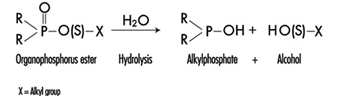
Alkyl phosphate metabolites.

The alkyl phosphate metabolites detectable in urine and the main parent compound from which they can originate are listed in table 5. Urinary alkyl phosphates are sensitive indicators of exposure to OP compounds: the excretion of these metabolites in urine is usually detectable at an exposure level at which plasma or erythrocyte cholinesterase inhibition cannot be detected. The urinary excretion of alkyl phosphates has been measured for different conditions of exposure and for various OP compounds (table 6). The existence of a relationship between external doses of OP and alkyl phosphate urinary concentrations has been established in a few studies. In some studies a significant relationship between cholinesterase activity and levels of alkyl phosphates in urine has also been demonstrated.

Table 5. Alkyl phosphates detectable in urine as metabolites of OP pesticides

Metabolite	Abbreviation	Principal parent compounds
Monomethylphosphate	MMP	Malathion, parathion
Dimethylphosphate	DMP	Dichlorvos, trichlorfon, mevinphos, malaoxon, dimethoate, fenchlorphos
Diethylphosphate	DEP	Paraoxon, demeton-oxon, diazinon-oxon, dichlorfenthion
Dimethylthiophosphate	DMTP	Fenitrothion, fenchlorphos, malathion, dimethoate
Diethylthiophosphate	DETP	Diazinon, demethon, parathion,fenchlorphos
Dimethyldithiophosphate	DMDTP	Malathion, dimethoate, azinphos-methyl
Diethyldithiophosphate	DEDTP	Disulfoton, phorate
Phenylphosphoric acid		Leptophos, EPN

Table 6. Examples of levels of urinary alkyl phosphates measured in various conditions of exposure to OP

Compound	Condition of exposure	Route of exposure	Metabolite concentrations¹ (mg/l)
Parathion²	Nonfatal poisoning	Oral	DEP = 0.5 DETP = 3.9
Disulfoton²	Formulators	Dermal/inhalation	DEP = 0.01-4.40 DETP = 0.01-1.57 DEDTP = <0.01-.05
Phorate²	Formulators	Dermal/inhalation	DEP = 0.02-5.14 DETP = 0.08-4.08 DEDTP = <0.01-0.43
Malathion³	Sprayers	Dermal	DMDTP = <0.01
Fenitrothion³	Sprayers	Dermal	DMP = 0.01-0.42 DMTP = 0.02-0.49
Monocrotophos⁴	Sprayers	Dermal/inhalation	DMP = <0.04-6.3/24 h

¹For abbreviations see table 27.12 [BMO12TE].
²Dillon and Ho 1987.
³Richter 1993.
⁴van Sittert and Dumas 1990.

Alkyl phosphates are usually excreted in urine within a short time. Samples collected soon after the end of the workday are suitable for metabolite determination.

The measurement of alkyl phosphates in urine requires a rather sophisticated analytical method, based on derivatization of the compounds and detection by gas-liquid chromatography (Shafik et al. 1973a; Reid and Watts 1981).

Hydrolytic residues.

p-Nitrophenol (PNP) is the phenolic metabolite of parathion, methylparathion and ethyl parathion, EPN. The measurement of PNP in urine (Cranmer 1970) has been widely used and has proven to be successful in evaluating exposure to parathion. Urinary PNP correlates well with the absorbed dose of parathion. With PNP urinary levels up to 2 mg/l, the absorption of parathion does not cause symptoms, and little or no reduction of cholinesterase activities is observed. PNP excretion occurs rapidly and urinary levels of PNP become insignificant 48 hours after exposure. Thus, urine samples should be collected soon after exposure.

Carbamates

Biological indicators of effect.

Carbamate pesticides include insecticides, fungicides and herbicides. Insecticidal carbamate toxicity is due to the inhibition of synaptic ACHE, while other mechanisms of toxicity are involved for herbicidal and fungicidal carbamates. Thus, only exposure to carbamate insecticides can be monitored through the assay of cholinesterase activity in red blood cells (ACHE) or plasma (PCHE). ACHE is usually more sensitive to carbamate inhibitors than PCHE. Cholinergic symptoms have been usually observed in carbamate-exposed workers with a blood ACHE activity lower than 70% of the individual baseline level (WHO 1982a).

Inhibition of cholinesterases by carbamates is rapidly reversible. Therefore, false negative results can be obtained if too much time elapses between exposure and biological sampling or between sampling and analysis. In order to avoid such problems, it is recommended that blood samples be collected and analysed within four hours after exposure. Preference should be given to the analytical methods that allow the determination of cholinesterase activity immediately after blood sampling, as discussed for organophosphates.

Biological indicators of exposure.

The measurement of urinary excretion of carbamate metabolites as a method to monitor human exposure has so far been applied only to few compounds and in limited studies. Table 7 summarizes the relevant data. Since carbamates are promptly excreted in the urine, samples collected soon after the end of exposure are suitable for metabolite determination. Analytical methods for the measurements of carbamate metabolites in urine have been reported by Dawson et al. (1964); DeBernardinis and Wargin (1982) and Verberk et al. (1990).

Table 7. Levels of urinary carbamate metabolites measured in field studies

Compound

Biological index

Condition of exposure

Environmental concentrations

Results

References

Carbaryl

a-naphthol

formulators

mixer/applicators

unexposed population

0.23–0.31 mg/m³

x=18.5 mg/l¹ , max. excretion rate = 80 mg/day

x=8.9 mg/l, range = 0.2–65 mg/l

range = 1.5–4 mg/l

WHO 1982a

Pirimicarb

metabolites I² and V³

applicators

range = 1–100 mg/l

Verberk et al. 1990

¹Systemic poisonings have been occasionally reported.
²2-dimethylamino-4-hydroxy-5,6-dimethylpyrimidine.
³2-methylamino-4-hydroxy-5,6-dimethylpyrimidine.
x = standard deviation.

Dithiocarbamates

Biological indicators of exposure.

Dithiocarbamates (DTC) are widely used fungicides, chemically grouped in three classes: thiurams, dimethyldithiocarbamates and ethylene-bis-dithiocarbamates.

Carbon disulphide (CS₂) and its main metabolite 2-thiothiazolidine-4-carboxylic acid (TTCA) are metabolites common to almost all DTC. A significant increase in urinary concentrations of these compounds has been observed for different conditions of exposure and for various DTC pesticides. Ethylene thiourea (ETU) is an important urinary metabolite of ethylene-bis-dithiocarbamates. It may also be present as an impurity in market formulations. Since ETU has been determined to be a teratogen and a carcinogen in rats and in other species and has been associated with thyroid toxicity, it has been widely applied to monitor ethylene-bis-dithiocarbamate exposure. ETU is not compound-specific, as it may be derived from maneb, mancozeb or zineb.

Measurement of the metals present in the DTC has been proposed as an alternative approach in monitoring DTC exposure. Increased urinary excretion of manganese has been observed in workers exposed to mancozeb (table 8).

Table 8. Levels of urinary dithiocarbamate metabolites measured in field studies

Compound	Biological index	Condition of exposure	Environmental concentrations* ± standard deviation	Results ± standard deviation	References
Ziram	Carbon disulphide (CS₂) TTCA¹	formulators formulators	1.03 ± 0.62 mg/m³	3.80 ± 3.70 mg/l 0.45 ± 0.37 mg/l	Maroni et al. 1992
Maneb/Mancozeb	ETU²	applicators		range = < 0.2–11.8 mg/l	Kurttio et al. 1990
Mancozeb	Manganese	applicators	57.2 mg/m³	pre-exposure: 0.32 ± 0.23 mg/g creatinine; post-exposure: 0.53 ± 0.34 mg/g creatinine	Canossa et al. 1993

* Mean result according to Maroni et al. 1992.
¹TTCA = 2-thiothiazolidine-4-carbonylic acid.
²ETU = ethylene thiourea.

CS₂, TTCA, and manganese are commonly found in urine of non-exposed subjects. Thus, the measurement of urinary levels of these compounds prior to exposure is recommended. Urine samples should be collected in the morning following the cessation of exposure. Analytical methods for the measurements of CS₂, TTCA and ETU have been reported by Maroni et al. (1992).

Synthetic Pyrethroids

Biological indicators of exposure.

Synthetic pyrethroids are insecticides similar to natural pyrethrins. Urinary metabolites suitable for application in biological monitoring of exposure have been identified through studies with human volunteers. The acidic metabolite 3-(2,2’-dichloro-vinyl)-2,2’-dimethyl-cyclopropane carboxylic acid (Cl₂CA) is excreted both by subjects orally dosed with permethrin and cypermethrin and the bromo-analogue (Br₂CA) by subjects treated with deltamethrin. In the volunteers treated with cypermethrin, a phenoxy metabolite, 4-hydroxy-phenoxy benzoic acid (4-HPBA), has also been identified. These tests, however, have not often been applied in monitoring occupational exposures because of the complex analytical techniques required (Eadsforth, Bragt and van Sittert 1988; Kolmodin-Hedman, Swensson and Akerblom 1982). In applicators exposed to cypermethrin, urinary levels of Cl₂CA have been found to range from 0.05 to 0.18 mg/l, while in formulators exposed to a-cypermethrin, urinary levels of 4-HPBA have been found to be lower than 0.02 mg/l.

A 24-hour urine collection period started after the end of exposure is recommended for metabolite determinations.

Organochlorines

Biological indicators of exposure.

Organochlorine (OC) insecticides were widely used in the 1950s and 1960s. Subsequently, the use of many of these compounds was discontinued in many countries because of their persistence and consequent contamination of the environment.

Biological monitoring of OC exposure can be carried out through the determination of intact pesticides or their metabolites in blood or serum (Dale, Curley and Cueto 1966; Barquet, Morgade and Pfaffenberger 1981). After absorption, aldrin is rapidly metabolized to dieldrin and can be measured as dieldrin in blood. Endrin has a very short half-life in blood. Therefore, endrin blood concentration is of use only in determining recent exposure levels. The determination of the urinary metabolite anti-12-hydroxy-endrin has also proven to be useful in monitoring endrin exposure (van Sittert and Tordoir 1987) .

Significant correlations between the concentration of biological indicators and the onset of toxic effects have been demonstrated for some OC compounds. Instances of toxicity due to aldrin and dieldrin exposure have been related to levels of dieldrin in blood above 200 μg/l. A blood lindane concentration of 20 μg/l has been indicated as the upper critical level as far as neurological signs and symptoms are concerned. No acute adverse effects have been reported in workers with blood endrin concentrations below 50 μg/l. Absence of early adverse effects (induction of liver microsomal enzymes) has been shown on repeated exposures to endrin at urinary anti-12-hydroxy-endrin concentrations below 130 μg/g creatinine and on repeated exposures to DDT at DDT or DDE serum concentrations below 250 μg/l.

OC may be found in low concentrations in the blood or urine of the general population. Examples of observed values are as follows: lindane blood concentrations up to 1 μg/l, dieldrin up to 10 μg/l, DDT or DDE up to 100 μg/l, and anti-12-hydroxy-endrin up to 1 μg/g creatinine. Thus, a baseline assessment prior to exposure is recommended.

For exposed subjects, blood samples should be taken immediately after the end of a single exposure. For conditions of long-term exposure, the time of collection of the blood sample is not critical. Urine spot samples for urinary metabolite determination should be collected at the end of exposure.

Triazines

Biological indicators of exposure.

The measurement of urinary excretion of triazinic metabolites and the unmodified parent compound has been applied to subjects exposed to atrazine in limited studies. Figure 2 shows the urinary excretion profiles of atrazine metabolites of a manufacturing worker with dermal exposure to atrazine ranging from 174 to 275 μmol/workshift (Catenacci et al. 1993). Since other chlorotriazines (simazine, propazine, terbuthylazine) follow the same biotransformation pathway of atrazine, levels of dealkylated triazinic metabolites may be determined to monitor exposure to all chlorotriazine herbicides.

Figure 2. Urinary excretion profiles of atrazine metabolites

The determination of unmodified compounds in urine may be useful as a qualitative confirmation of the nature of the compound that has generated the exposure. A 24–hour urine collection period started at the beginning of exposure is recommended for metabolite determination.

Recently, by using an enzyme-linked immunosorbent assay (ELISA test), a mercapturic acid conjugate of atrazine has been identified as its major urinary metabolite in exposed workers. This compound has been found in concentrations at least 10 times higher than those of any dealkylated products. A relationship between cumulative dermal and inhalation exposure and total amount of the mercapturic acid conjugate excreted over a 10-day period has been observed (Lucas et al. 1993).

Coumarin Derivatives

Biological indicators of effect.

Coumarin rodenticides inhibit the activity of the enzymes of the vitamin K cycle in the liver of mammals, humans included (figure 3), thus causing a dose-related reduction of the synthesis of vitamin K-dependent clotting factors, namely factor II (prothrombin), VII, IX, and X. Anticoagulant effects appear when plasma levels of clotting factors have dropped below approximately 20% of normal.

Figure 3. Vitamin K cycle

These vitamin K antagonists have been grouped into so-called “first generation” (e.g., warfarin) and “second generation” compounds (e.g., brodifacoum, difenacoum), the latter characterized by a very long biological half-life (100 to 200 days).

The determination of prothrombin time is widely used in monitoring exposure to coumarins. However, this test is sensitive only to a clotting factor decrease of approximately 20% of normal plasma levels. The test is not suitable for detection of early effects of exposure. For this purpose, the determination of the prothrombin concentration in plasma is recommended.

In the future, these tests might be replaced by the determination of coagulation factor precursors (PIVKA), which are substances detectable in blood only in the case of blockage of the vitamin K cycle by coumarins.

With conditions of prolonged exposure, the time of blood collection is not critical. In cases of acute overexposure, biological monitoring should be carried out for at least five days after the event, in view of the latency of the anticoagulant effect. To increase the sensitivity of these tests, the measurement of baseline values prior to exposure is recommended.

Biological indicators of exposure.

The measurement of unmodified coumarins in blood has been proposed as a test to monitor human exposure. However, experience in applying these indices is very limited mainly because the analytical techniques are much more complex (and less standardized) in comparison with those required to monitor the effects on the coagulation system (Chalermchaikit, Felice and Murphy 1993).

Phenoxy Herbicides

Biological indicators of exposure.

Phenoxy herbicides are scarcely biotransformed in mammals. In humans, more than 95% of a 2,4-dichlorophenoxyacetic acid (2,4-D) dose is excreted unchanged in urine within five days, and 2,4,5-trichlorophenoxyacetic acid (2,4,5-T) and 4-chloro-2-methylphenoxyacetic acid (MCPA) are also excreted mostly unchanged via urine within a few days after oral absorption. The measurement of unchanged compounds in urine has been applied in monitoring occupational exposure to these herbicides. In field studies, urinary levels of exposed workers have been found to range from 0.10 to 8 μg/l for 2,4-D, from 0.05 to 4.5 μg/l for 2,4,5-T and from below 0.1 μg/l to 15 μg/l for MCPA. A 24-hour period of urine collection starting at the end of exposure is recommended for the determination of unchanged compounds. Analytical methods for the measurements of phenoxy herbicides in urine have been reported by Draper (1982).

Quaternary Ammonium Compounds

Biological indicators of exposure.

Diquat and paraquat are herbicides scarcely biotransformed by the human organism. Because of their high water solubility, they are readily excreted unchanged in urine. Urine concentrations below the analytical detection limit (0.01 μg/l) have been often observed in paraquat exposed workers; while in tropical countries, concentrations up to 0.73 μg/l have been measured after improper paraquat handling. Urinary diquat concentrations lower than the analytical detection limit (0.047 μg/l) have been reported for subjects with dermal exposures from 0.17 to 1.82 μg/h and inhalation exposures lower than 0.01 μg/h. Ideally, 24 hours sampling of urine collected at the end of exposure should be used for analysis. When this is impractical, a spot sample at the end of the workday can be used.

Determination of paraquat levels in serum is useful for prognostic purposes in case of acute poisoning: patients with serum paraquat levels up to 0.1 μg/l twenty-four hours after ingestion are likely to survive.

The analytical methods for paraquat and diquat determination have been reviewed by Summers (1980).

Miscellaneous Pesticides

4,6-Dinitro-o-cresol (DNOC).

DNOC is an herbicide introduced in 1925, but the use of this compound has been progressively decreased due to its high toxicity to plants and to humans. Since blood DNOC concentrations correlate to a certain extent with the severity of adverse health effects, the measure of unchanged DNOC in blood has been proposed for monitoring occupational exposures and for the evaluation of the clinical course of poisonings.

Pentachlorophenol.

Pentachlorophenol (PCP) is a wide-spectrum biocide with pesticidal action against weeds, insects, and fungi. Measurements of blood or urinary unchanged PCP have been recommended as suitable indices in monitoring occupational exposures (Colosio et al. 1993), because these parameters are significantly correlated with PCP body burden. In workers with prolonged exposure to PCP the time of blood collection is not critical, while urine spot samples should be collected on the morning after exposure.

A multiresidue method for the measurement of halogenated and nitrophenolic pesticides has been described by Shafik et al.(1973b).

Other tests proposed for the biological monitoring of pesticide exposure are listed in table 9.

Table 9. Other indices proposed in the literature for the biological monitoring of pesticide exposure

Compound	Biological index
	Urine	Blood
Bromophos	Bromophos	Bromophos
Captan	Tetrahydrophtalimide
Carbofuran	3-Hydroxycarbofuran
Chlordimeform	4-Chloro-o-toluidine derivatives
Chlorobenzilate	p,p-1-Dichlorobenzophenone
Dichloropropene	Mercapturic acid metabolites
Fenitrothion	p-Nitrocresol
Ferbam		Thiram
Fluazifop-Butyl	Fluazifop
Flufenoxuron		Flufenoxuron
Glyphosate	Glyphosate
Malathion	Malathion	Malathion
Organotin compounds	Tin	Tin
Trifenomorph	Morpholine, triphenylcarbinol
Ziram		Thiram

Conclusions

Biological indicators for monitoring pesticide exposure have been applied in a number of experimental and field studies.

Some tests, such as those for cholinesterase in blood or for selected unmodified pesticides in urine or blood, have been validated by extensive experience. Biological exposure limits have been proposed for these tests (table 10). Other tests, in particular those for blood or urinary metabolites, suffer from greater limitations because of analytical difficulties or because of limitations in interpretation of results.

Table 10. Recommended biological limit values (as of 1996)

Compound	Biological index	BEI¹	BAT²	HBBL³	BLV⁴
ACHE inhibitors	ACHE in blood	70%	70%	70%,
DNOC	DNOC in blood			20 mg/l,
Lindane	Lindane in blood		0.02mg/l	0.02mg/l
Parathion	PNP in urine	0.5mg/l	0.5mg/l
Pentachlorophenol (PCP)	PCP in urine PCP in plasma	2 mg/l 5 mg/l	0.3mg/l 1 mg/l
Dieldrin/Aldrin	Dieldrin in blood				100 mg/l
Endrin	Anti-12-hydroxy-endrin in urine				130 mg/l
DDT	DDT and DDEin serum				250 mg/l
Coumarins	Prothrombin time in plasma Prothrombin concentration in plasma				10% above baseline 60% of baseline
MCPA	MCPA in urine				0.5 mg/l
2,4-D	2,4-D in urine				0.5 mg/l

¹Biological exposure indices (BEIs) are recommended by the American Conference of Governmental Industrial Hygienists (ACGIH 1995).
²Biological tolerance values (BATs) are recommended by the German Commission for the Investigation of Health Hazards of Chemical Compounds in the Work Area (DFG 1992).
³Health-based biological limits (HBBLs) are recommended by a WHO Study Group (WHO 1982a).
⁴Biological limit values (BLVs) are proposed by a Study Group of the Scientific Committee on Pesticides of the International Commission on Occupational Health (Tordoir et al. 1994). Assessment of working conditions is called for if this value is exceeded.

This field is in rapid development and, given the enormous importance of using biological indicators to assess exposure to these substances, new tests will be continuously developed and validated.

Back

Published in 27. Biological Monitoring

Monday, 28 February 2011 20:25

Genotoxic Chemicals

Human biological monitoring uses samples of body fluids or other easily obtainable biological material for the measurement of exposure to specific or nonspecific substances and/or their metabolites or for the measurement of the biological effects of this exposure. Biological monitoring allows one to estimate total individual exposure through different exposure pathways (lungs, skin, gastrointestinal tract) and different sources of exposure (air, diet, lifestyle or occupation). It is also known that in complex exposure situations, which are very often encountered in workplaces, different exposing agents may interact with one another, either enhancing or inhibiting the effects of the individual compounds. And since individuals differ in their genetic constitution, they exhibit variability in their response to chemical exposures. Thus, it may be more reasonable to look for early effects directly in the exposed individuals or groups than to try to predict potential hazards of the complex exposure patterns from data pertaining to single compounds. This is an advantage of genetic biomonitoring for early effects, an approach employing techniques that focus on cytogenetic damage, point mutations, or DNA adducts in surrogate human tissue (see the article “General principles” in this chapter).

What Is Genotoxicity?

Genotoxicity of chemical agents is an intrinsic chemical character, based on the agent’s electrophilic potential to bind with such nucleophilic sites in the cellular macromolecules as deoxyribonucleic acid, DNA, the carrier of hereditary information. Genotoxicity is thus toxicity manifested in the genetic material of cells.

The definition of genotoxicity, as discussed in a consensus report (IARC 1992), is broad, and includes both direct and indirect effects in DNA: (1) the induction of mutations (gene, chromosomal, genomial, recombinational) that at the molecular level are similar to events known to be involved in carcinogenesis, (2) indirect surrogate events associated with mutagenesis (e.g., unscheduled DNA synthesis (UDS) and sister chromatid exchange (SCE), or (3) DNA damage (e.g., the formation of adducts), which may eventually lead to mutations.

Genotoxicity, Mutagenicity And Carcinogenicity

Mutations are permanent hereditary changes in the cell lines, either horizontally in the somatic cells or vertically in the germinal (sex) cells of the body. That is, mutations may affect the organism itself through changes in body cells, or they may be passed on to other generations through alteration of the sex cells. Genotoxicity thus preceeds mutagenicity although most of genotoxicity is repaired and is never expressed as mutations. Somatic mutations are induced at the cellular level and in the event that they lead to cell death or malignancies, may become manifest as various disorders of tissues or of the organism itself. Somatic mutations are thought to be related to ageing effects or to the induction of atherosclerotic plaques (see figure 1 and the chapter on Cancer).

Figure 1. Schematic view of the scientific paradigm in genetic toxicology and human health effects

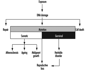
Mutations in the germ cell line may be transferred to the zygote—the fertilized egg cell—and be expressed in the offspring generation (see also the chapter Reproductive System). The most important mutational disorders found in the newborn are induced by malsegregation of chromosomes during gametogenesis (the development of germ cells) and result in severe chromosomal syndromes (e.g., trisomy 21 or Down’s syndrome, and monosomy X or Turner’s syndrome).

The paradigm of genotoxicology from exposure to anticipated effects may be simplified as shown in figure 1.

The relationship of genotoxicity to carcinogenicity is well supported by various indirect research facts, as shown in figure 2.

Figure 2. The interrelationships of genotoxicity and carcinogenicity

This correlation provides the basis for applying biomarkers of genotoxicity to be used in human monitoring as indicators of cancer hazard.

Genetic Toxicity in Hazard Identification

The role of genetic changes in carcinogenesis underscores the importance of genetic toxicity testing in the identification of potential carcinogens. Various short-term test methods have been developed which are able to detect some of the endpoints in genotoxicity supposedly relevant in carcinogenesis.

Several extensive surveys have been performed to compare the carcinogenicity of chemicals with results obtained by examining them in short-term tests. The general conclusion has been that since no single validated test can provide information on all of the above-mentioned genetic end-points; it is necessary to test each chemical in more than one assay. Also, the value of short-term tests of genetic toxicity for prediction of chemical carcinogenicity has been discussed and reviewed repeatedly. On the basis of such reviews, a working group at the International Agency for Research on Cancer (IARC) concluded that most human carcinogens give positive results in routinely used short-term tests such as the Salmonella assay and the chromosome aberration assays (table 1). However, it must be realized that the epigenetic carcinogens—such as hormonally active compounds which can increase genotoxic activity without themselves being genotoxic—cannot be detected by short-term tests, which measure only the intrinsic genotoxic activity of a substance.

Table 1. Genotoxicity of chemicals evaluated in Supplements 6 and 7 to the IARC Monographs (1986)

Carcinogenicity classification	Ratio of evidence for genotoxicity/carcinogenicity	%
1: human carcinogens	24/30	80
2A: probable human carcinogens	14/20	70
2B: possible human carcinogens	72/128	56
3: not classifiable	19/66	29

Genetic Biomonitoring

Genetic monitoring utilizes genetic toxicology methods for biological monitoring of genetic effects or assessment of genotoxic exposure in a group of individuals with defined exposure at a worksite or through environment or lifestyle. Thus, genetic monitoring has the potential for early identification of genotoxic exposures in a group of persons and enables identification of high-risk populations and thus priorities for intervention. Use of predictive biomarkers in an exposed population is warranted to save time (as compared with epidemiological techniques) and to prevent unnecessary end effects, namely cancer (figure 3).

Figure 3. The predictiveness of biomarkers enables preventive actions to be taken to decrease risks to health in human populations

The methods currently used for biomonitoring of genotoxic exposure and early biological effects are listed in table 2. The samples used for biomonitoring must meet several criteria, including the necessity that they be both easily obtainable and comparable with the target tissue.

Table 2. Biomarkers in genetic monitoring of genotoxicity exposure and the most commonly used cell/tissue samples.

Marker of genetic monitoring	Cell/tissue samples
Chromosomal aberrations (CA)	Lymphocytes
Sister chromatid exchanges (SCE)	Lymphocytes
Micronuclei (MN)	Lymphocytes
Point mutations (e.g., HPRT gene)	Lymphocytes and other tissues
DNA adducts	DNA isolated from cells/tissues
Protein adducts	Haemoglobin, albumin
DNA strand breaks	DNA isolated from cells/tissues
Oncogene activation	DNA or specific proteins isolated
Mutations/oncoproteins	Various cells and tissues
DNA repair	Isolated cells from blood samples

The types of molecularly recognisable DNA damage include the formation of DNA adducts and reorganization of the DNA sequence. These kinds of damage can be detected by measurements of DNA adducts using various techniques, for example, either 32P-postlabelling or the detection of monoclonal antibodies to DNA adducts. Measurement of DNA strand breaks is conventionally carried out using alkaline elution or unwinding assays. Mutations may be detected by sequencing the DNA of a specific gene, for example, the HPRT gene.

Several methodological reports have appeared that discuss the techniques of table 2 in detail (CEC 1987; IARC 1987, 1992, 1993).

Genotoxicity can also be monitored indirectly through the measurement of protein adducts, that is, in haemoglobin instead of DNA, or the monitoring of DNA repair activity. As a measuring strategy, the monitoring activity may be either one time or continuous. In all cases the results must be applied to the development of safe working conditions.

Cytogenetic Biomonitoring

A theoretical and empirical rationale links cancer to chromosome damage. Mutational events altering the activity or expression of growth-factor genes are key steps in carcinogenesis. Many types of cancers have been associated with specific or nonspecific chromosomal aberrations. In several hereditary human diseases, chromosome instability is associated with increased susceptibility to cancer.

Cytogenetic surveillance of people exposed to carcinogenic and/or mutagenic chemicals or radiation can bring to light effects on the genetic material of the individuals concerned. Chromosomal aberration studies of people exposed to ionizing radiation have been applied for biological dosimetry for decades, but well-documented positive results are as yet available only for a limited number of chemical carcinogens.

Microscopically recognizable chromosomal damage includes both structural chromosomal aberrations (CA), in which a gross change in the morphology (shape) of a chromosome has occurred, and by sister chromatid exchanges (SCE). SCE is the symmetrical exchange of chromosomal materials between two sister chromatids. Micronuclei (MN) can arise either from acentric chromosome fragments or from lagging whole chromosomes. These types of changes are illustrated in figure 4.

Figure 4. Human lymphocyte chromosomes at metaphase, revealing an induced chromosome mutation (arrow pointing to an acentric fragment)

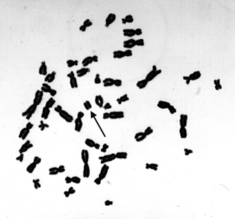
Peripheral blood lymphocytes in humans are suitable cells to be used in surveillance studies because of their easy accessibility and because they can integrate exposure over a relatively long lifespan. Exposure to a variety of chemical mutagens may result in increased frequencies of CAs and/or SCEs in blood lymphocytes of exposed individuals. Also, the extent of damage is roughly correlated with exposure, although this has been shown with only a few chemicals.

When cytogenetic tests on peripheral blood lymphocytes show that the genetic material has been damaged, the results can be used to estimate risk only at the level of the population. An increased frequency of CAs in a population should be considered an indication of increased risk to cancer, but cytogenetic tests do not, as such, allow individual risk prediction of cancer.

The health significance of somatic genetic damage as seen through the narrow window of a sample of peripheral blood lymphocytes has little or no significance to the health of an individual, since most of the lymphocytes carrying genetic damage die and are replaced.

Problems and their Control in Human Biomonitoring Studies

Rigorous study design is necessary in the application of any human biomonitoring method, since many interindividual factors that are not related to the specific chemical exposure(s) of interest may affect the biological responses studied. Since human biomonitoring studies are tedious and difficult in many respects, careful preplanning is very important. In performing human cytogenetic studies, experimental confirmation of the chromosome damaging potential of the exposing agent(s) should always be an experimental prerequisite.

In cytogenetic biomonitoring studies, two major types of variations have been documented. The first includes technical factors associated with slide-reading discrepancies and with culture conditions, specifically with the type of medium, temperature, and concentration of chemicals (such as bromodeoxyuridine or cytochalasin-B). Also, sampling times can alter chromosome aberration yields, and possibly also findings of SCE incidence, through changes in subpopulations of T- and B-lymphocytes. In micronucleus analyses, methodological differences (e.g., use of binucleated cells induced by cytochalasin-B) quite clearly affect the scoring results.

The lesions induced in the DNA of lymphocytes by chemical exposure that lead to formation of structural chromosome aberrations, sister chromatid exchange, and micronuclei must persist in vivo until the blood is withdrawn and then in vitro until the cultured lymphocyte begins DNA synthesis. It is, therefore, important to score cells directly after the first division (in the case of chromosome aberrations or micronuclei) or after the second division (sister chromatid exchanges) in order to obtain the best estimate of induced damage.

Scoring constitutes an extremely important element in cytogenetic biomonitoring. Slides must be randomized and coded to avoid scorer bias as far as possible. Consistent scoring criteria, quality control and standardized statistical analyses and reporting should be maintained. The second category of variability is due to conditions associated with the subjects, such as age, sex, medication and infections. Individual variations can also be caused by genetic susceptibility to environmental agents.

It is critical to obtain a concurrent control group that is matched as closely as possible on internal factors such as sex and age as well as on factors such as smoking status, viral infections and vaccinations, alcohol and drug intake, and exposure to x-rays. Additionally, it is necessary to obtain qualitative (job category, years exposed) and quantitative (e.g., breathing zone air samples for chemical analysis and specific metabolites, if possible) estimates or exposure to the putative genotoxic agent(s) in the workplace. Special consideration should be paid to proper statistical treatment of the results.

Relevancy of genetic biomonitoring to cancer risk assessment

The number of agents repeatedly shown to induce cytogenetic changes in humans is still relatively limited, but most known carcinogens induce damage in lymphocyte chromosomes.

The extent of damage is a function of exposure level, as has been shown to be the case with, for example, vinyl chloride, benzene, ethylene oxide, and alkylating anticancer agents. Even if the cytogenetic end points are not very sensitive or specific as regards the detection of exposures occurring in present-day occupational settings, positive results of such tests have often prompted implementation of hygienic controls even in the absence of direct evidence relating somatic chromosomal damage to adverse health outcomes.

Most experience with application of cytogenetic biomonitoring derives from “high exposure” occupational situations. Very few exposures have been confirmed by several independent studies, and most of these have been performed using chromosomal aberration biomonitoring. The database of the International Agency for Research on Cancer lists in its updated volumes 43–50 of the IARC Monographs a total of 14 occupational carcinogens in groups 1, 2A or 2B, for which there is positive human cytogenetic data available that are in most cases supported by corresponding animal cytogenetics (table 3). This limited database suggests that there is a tendency for carcinogenic chemicals to be clastogenic, and that clastogenicity tends to be associated with known human carcinogens. Quite clearly, however, not all carcinogens induce cytogenetic damage in humans or experimental animals in vivo. Cases in which the animal data are positive and the human findings are negative may represent differences in exposure levels. Also, the complex and long-term human exposures at work may not be comparable with short-term animal experiments.

Table 3. Proven, probable and possible human carcinogens for which occupational exposure exists and for which cytogenetic end points have been measured in both humans and experimental animals

	Cytogenic findings¹
	Humans			Animals
Agent/exposure	CA	SCE	MN	CA	SCE	MN
GROUP 1, Human carcinogens
Arsenic and arsenic compounds	?	?		+		+
Asbestos		?		–		–
Benzene	+			+	+	+
Bis(chloromethyl)ether and chloromethyl methyl ether (technical grade)	(+)			–
Cyclophosphamide	+	+		+	+	+
Hexavalent chromium compounds	+	+		+	+	+
Melphalan	+	+		+
Nickel compounds	+	–		?
Radon	+			–
Tobacco smoke	+	+	+		+
Vinyl chloride	+	?		+	+	+
GROUP 2A, Probable human carcinogens
Acrylonitrile	–			–		–
Adriamycin	+	+		+	+	+
Cadmium and cadmium compounds	–	(–)		–
Cisplatin		+		+	+
Epichlorohydrin	+			?	+	–
Ethylene dibromide	–	–		–	+	–
Ethylene oxide	+	+	+	+	+	+
Formaldehyde	?	?		–		–
GROUP 2B, Possible human carcinogens
Chlorophenoxy herbicides (2,4-D and 2,4,5-T)	–	–		+	+	–
DDT	?			+		–
Dimethylformamide	(+)				–	–
Lead compounds	?	?		?	–	?
Styrene	+	?	+	?	+	+
2,3,7,8-Tetrachlorodibenzo-para-dioxin	?			–	–	–
Welding fumes	+	+		–	–

¹CA, chromosomal aberration; SCE, sister chromatid exchange; MN, micronuclei.
(–) = negative relationship for one study;                      – = negative relationship;
(+) = positive relationship for one study;                       + = positive relationship;
? = inconclusive;                                              blank area = not studied

Source: IARC, 1987; updated through volumes 43–50 of IARC monographs.

Studies of genotoxicity in exposed humans include various end points other than chromosomal end points, such as DNA damage, DNA repair activity, and adducts in DNA and in proteins. Some of these end points may be more relevant than others for the prediction of carcinogenic hazard. Stable genetic changes (e.g., chromosomal rearrangements, deletions, and point mutations) are highly relevant, since these types of damage are known to be related to carcinogenesis. The significance of DNA adducts is dependent upon their chemical identification and evidence that they result from the exposure. Some endpoints, such as SCE, UDS, SSB, DNA strand breakage, are potential indicators and/or markers of genetic events; however, their value is reduced in the absence of a mechanistic understanding of their ability to lead to genetic events. Clearly, the most relevant genetic marker in humans would be the induction of a specific mutation that has been directly associated with cancer in rodents exposed to the agent under study (figure 5).

Figure 5. Relevance of different genetic biomonitoring effects for potential cancer risk

Ethical Considerations for Genetic Biomonitoring

Rapid advances in molecular genetic techniques, the enhanced speed of sequencing of the human genome, and the identification of the role of tumour suppressor genes and proto-oncogenes in human carcinogenesis, raise ethical issues in the interpretation, communication, and use of this kind of personal information. Quickly improving techniques for the analysis of human genes will soon allow the identification of yet more inherited susceptibility genes in healthy, asymptomatic individuals (US Office of Technology Assessment 1990), lending themselves to be used in genetic screening.

Many questions of social and ethical concern will be raised if the application of genetic screening soon becomes a reality. Already at present roughly 50 genetic traits of metabolism, enzyme polymorphisms, and DNA repair are suspected for specific disease sensitivities, and a diagnostic DNA test is available for about 300 genetic diseases. Should any genetic screening at all be performed at the workplace? Who is to decide who will undergo testing, and how will the information be used in employment decisions? Who will have access to the information obtained from genetic screening, and how will the results be communicated to the person(s) involved? Many of these questions are strongly linked to social norms and prevailing ethical values. The main objective must be the prevention of disease and human suffering, but respect must be accorded to the individual’s own will and ethical premises. Some of the relevant ethical questions which must be answered well before the outset of any workplace biomonitoring study are given in table 4 and are also discussed in the chapter Ethical Issues.

Table 4. Some ethical principles relating to the need to know in occupational genetic biomonitoring studies

	Groups to whom information is given
Information given	Persons studied	Occupational health unit	Employer
What is being studied
Why is the study performed
Are there risks involved
Confidentiality issues
Preparedness for possible hygienic improvements, exposure reductions indicated

Time and effort must be put into the planning phase of any genetic biomonitoring study, and all necessary parties—the employees, employers, and the medical personnel of the collaborating workplace—must be well-informed before the study, and the results made known to them after the study as well. With proper care and reliable results, genetic biomonitoring can help to ensure safer workplaces and improve workers’ health.

Back

Published in 27. Biological Monitoring

Monday, 28 February 2011 20:21

Organic Solvents

Introduction

Organic solvents are volatile and generally soluble in body fat (lipophilic), although some of them, e.g., methanol and acetone, are water soluble (hydrophilic) as well. They have been extensively employed not only in industry but in consumer products, such as paints, inks, thinners, degreasers, dry-cleaning agents, spot removers, repellents, and so on. Although it is possible to apply biological monitoring to detect health effects, for example, effects on the liver and the kidney, for the purpose of health surveillance of workers who are occupationally exposed to organic solvents, it is best to use biological monitoring instead for “exposure” monitoring in order to protect the health of workers from the toxicity of these solvents, because this is an approach sensitive enough to give warnings well before any health effects may occur. Screening workers for high sensitivity to solvent toxicity may also contribute to the protection of their health.

Summary of Toxicokinetics

Organic solvents are generally volatile under standard conditions, although the volatility varies from solvent to solvent. Thus, the leading route of exposure in industrial settings is through inhalation. The rate of absorption through the alveolar wall of the lungs is much higher than that through the digestive tract wall, and a lung absorption rate of about 50% is considered typical for many common solvents such as toluene. Some solvents, for example, carbon disulphide and N,N-dimethylformamide in the liquid state, can penetrate intact human skin in amounts large enough to be toxic.

When these solvents are absorbed, a portion is exhaled in the breath without any biotransformation, but the greater part is distributed in organs and tissues rich in lipids as a result of their lipophilicity. Biotransformation takes place primarily in the liver (and also in other organs to a minor extent), and the solvent molecule becomes more hydrophilic, typically by a process of oxidation followed by conjugation, to be excreted via the kidney into the urine as metabolite(s). A small portion may be eliminated unchanged in the urine.

Thus, three biological materials, urine, blood and exhaled breath, are available for exposure monitoring for solvents from a practical viewpoint. Another important factor in selecting biological materials for exposure monitoring is the speed of disappearance of the absorbed substance, for which the biological half-life, or the time needed for a substance to diminish to one-half its original concentration, is a quantitative parameter. For example, solvents will disappear from exhaled breath much more rapidly than corresponding metabolites from urine, meaning they have a much shorter half-life. Within urinary metabolites, the biological half-life varies depending on how quickly the parent compound is metabolised, so that sampling time in relation to exposure is often of critical importance (see below). A third consideration in choosing a biological material is the specificity of the target chemical to be analysed in relation to the exposure. For example, hippuric acid is a long-used marker of exposure to toluene, but it is not only formed naturally by the body, but can also be derived from non-occupational sources such as some food additives, and is no longer considered a reliable marker when toluene exposure is low (less than 50 cm³/m³). Generally speaking, urinary metabolites have been most widely used as indicators of exposure to various organic solvents. Solvent in blood is analysed as a qualitative measure of exposure because it usually remains in the blood a shorter time and is more reflective of acute exposure, whereas solvent in exhaled breath is difficult to use for estimation of average exposure because the concentration in breath declines so rapidly after cessation of exposure. Solvent in urine is a promising candidate as a measure of exposure, but it needs further validation.

Biological Exposure Tests for Organic Solvents

In applying biological monitoring for solvent exposure, sampling time is important, as indicated above. Table 1 shows recommended sampling times for common solvents in the monitoring of everyday occupational exposure. When the solvent itself is to be analysed, attention should be paid to preventing possible loss (e.g., evaporation into room air) as well as contamination (e.g., dissolving from room air into the sample) during the sample handling process. In case the samples need to be transported to a distant laboratory or to be stored before analysis, care should be exercised to prevent loss. Freezing is recommended for metabolites, whereas refrigeration (but no freezing) in an airtight container without an air space (or more preferably, in a headspace vial) is recommended for analysis of the solvent itself. In chemical analysis, quality control is essential for reliable results (for details, see the article “Quality assurance” in this chapter). In reporting the results, ethics should be respected (see chapter Ethical Issues elsewhere in the Encyclopaedia).

Table 1. Some examples of target chemicals for biological monitoring and sampling time

Solvent	Target chemical	Urine/blood	Sampling time¹
Carbon disulphide	2-Thiothiazolidine-4-carboxylicacid	Urine	Th F
N,N-Dimethyl-formamide	N-Methylformamide	Urine	M Tu W Th F
2-Ethoxyethanol and its acetate	Ethoxyacetic acid	Urine	Th F (end of last workshift)
Hexane	2,4-Hexanedione Hexane	Urine Blood	M Tu W Th F confirmation of exposure
Methanol	Methanol	Urine	M Tu W Th F
Styrene	Mandelic acid Phenylglyoxylic acid Styrene	Urine Urine Blood	Th F Th F confirmation of exposure
Toluene	Hippuric acid o-Cresol Toluene Toluene	Urine Urine Blood Urine	Tu W Th F Tu W Th F confirmation of exposure Tu W Th F
Trichloroethylene	Trichloroacetic acid (TCA) Total trichloro- compounds (sum of TCA and free and conjugated trichloroethanol) Trichloroethylene	Urine Urine Blood	Th F Th F confirmation of exposure
Xylenes²	Methylhippuric acids Xylenes	Urine Blood	Tu W Th F Tu W Th F

¹ End of workshift unless otherwise noted: days of week indicate preferred sampling days.
² Three isomers, either separately or in any combination.

Source: Summarized from WHO 1996.

Anumber of analytical procedures are established for many solvents. Methods vary depending on the target chemical, but most of the recently developed methods use gas chromatography (GC) or high-performance liquid chromatography (HPLC) for separation. Use of an autosampler and data processor is recommended for good quality control in chemical analysis. When a solvent itself in blood or in urine is to be analysed, an application of headspace technique in GC (headspace GC) is very convenient, especially when the solvent is volatile enough. Table 2 outlines some examples of the methods established for common solvents.

Table 2. Some examples of analytical methods for biological monitoring of exposure to organic solvents

Solvent	Target chemical	Blood/urine	Analytical method
Carbon disulphide	2-Thiothiazolidine-4- carboxylic acid	Urine	High performance liquid chromatograph with ultraviolet detection (UV-HPLC)
N,N-Dimethylformamide	N-Methylformamide	Urine	Gas chromatograph with flame thermionic detection (FTD-GC)
2-Ethoxyethanol and its acetate	Ethoxyacetic acid	Urine	Extraction, derivatization and gas chromatograph with flame ionization detection (FID-GC)
Hexane	2,4-Hexanedione Hexane	Urine Blood	Extraction, (hydrolysis) and FID-GC Head-space FID-GC
Methanol	Methanol	Urine	Head-space FID-GC
Styrene	Mandelic acid Phenylglyoxylic acid Styrene	Urine Urine Blood	Desalting and UV-HPLC Desalting and UV-HPLC Headspace FID-GC
Toluene	Hippuric acid o-Cresol Toluene Toluene	Urine Urine Blood Urine	Desalting and UV-HPLC Hydrolysis, extraction and FID-GC Headspace FID-GC Headspace FID-GC
Trichloroethylene	Trichloroacetic acid (TCA) Total trichloro-compounds (sum of TCA and freeand conjugated trichloroethanol) Trichloroethylene	Urine Urine Blood	Colorimetry or esterification and gas chromatograph with electron capture detection (ECD-GC) Oxidation and colorimetry, or hydrolysis, oxidation, esterification and ECD-GC Headspace ECD-GC
Xylenes	Methylhippuric acids (three isomers, either separately orin combination)	Urine	Headspace FID-GC

Source: Summarized from WHO 1996.

Evaluation

A linear relationship of the exposure indicators (listed in table 2) with the intensity of exposure to corresponding solvents may be established either through a survey of workers occupationally exposed to solvents, or by experimental exposure of human volunteers. Accordingly, the ACGIH (1994) and the DFG (1994), for example, have established the biological exposure index (BEI) and the biological tolerance value (BAT), respectively, as the values in the biological samples which are equivalent to the occupational exposure limit for airborne chemicals—that is, threshold limit value (TLV) and maximum workplace concentration (MAK), respectively. It is known, however, that the level of the target chemical in samples obtained from non-exposed people may vary, reflecting, for example, local customs (e.g., food), and that ethnic differences may exist in solvent metabolism. It is therefore desirable to establish limit values through the study of the local population of concern.

In evaluating the results, non-occupational exposure to the solvent (e.g., via use of solvent-containing consumer products or intentional inhalation) and exposure to chemicals which give rise to the same metabolites (e.g., some food additives) should be carefully excluded. In case there is a wide gap between the intensity of vapour exposure and the biological monitoring results, the difference may indicate the possibility of skin absorption. Cigarette smoking will suppress the metabolism of some solvents (e.g., toluene), whereas acute ethanol intake may suppress methanol metabolism in a competitive manner.

Back

Published in 27. Biological Monitoring

Monday, 28 February 2011 20:15

Metals and organometallic compounds

Toxic metals and organometallic compounds such as aluminium, antimony, inorganic arsenic, beryllium, cadmium, chromium, cobalt, lead, alkyl lead, metallic mercury and its salts, organic mercury compounds, nickel, selenium and vanadium have all been recognized for some time as posing potential health risks to exposed persons. In some cases, epidemiological studies on relationships between internal dose and resulting effect/response in occupationally exposed workers have been studied, thus permitting the proposal of health-based biological limit values (see table 1).

Table 1. Metals: Reference values and biological limit values proposed by the American Conference of Governmental Industrial Hygienists (ACGIH), Deutsche Forschungsgemeinschaft (DFG), and Lauwerys and Hoet (L and H)

Metal	Sample	Reference¹ values*	ACGIH (BEI) limit²	DFG (BAT) limit³	L and H limit⁴ (TMPC)
Aluminium	Serum/plasma Urine	<1 μg/100 ml <30 μg/g		200 μg/l (end of shift)	150 μg/g (end of shift)
Antimony	Urine	<1 μg/g			35 μg/g (end of shift)
Arsenic	Urine (sum of inorganic arsenic and methylated metabolites)	<10 μg/g	50 μg/g (end of workweek)		50 μg/g (if TWA: 0.05 mg/m³ ); 30 μg/g (if TWA: 0.01 mg/m³ ) (end of shift)
Beryllium	Urine	<2 μg/g
Cadmium	Blood Urine	<0.5 μg/100 ml <2 μg/g	0.5 μg/100 ml 5 μg/g	1.5 μg/100 ml 15 μg/l	0.5 μg/100 ml 5 μg/g
Chromium (soluble compounds)	Serum/plasma Urine	<0.05 μg/100 ml <5 μg/g	30 μg/g (end of shift, end of workweek); 10 μg/g (increase during shift)		30 μg/g (end of shift)
Cobalt	Serum/plasma Blood Urine	<0.05 μg/100 ml <0.2 μg/100 ml <2 μg/g	0.1 μg/100 ml (end of shift, end of workweek) 15 μg/l (end of shift, end of workweek)	0.5 μg/100 ml (EKA) 60 μg/l (EKA)	30 μg/g (end of shift, end of workweek)
Lead	Blood (lead) ZPP in blood Urine (lead) ALA urine	<25 μg/100 ml <40 μg/100 ml blood <2.5μg/g Hb <50 μg/g <4.5 mg/g	30 μg/100 ml (not critical)	female <45 years: 30 μg/100 ml male: 70 μg/100 ml female <45 years: 6 mg/l; male: 15 mg/l	40 μg/100 ml 40 μg/100 ml blood or 3 μg/g Hb 50 μg/g 5 mg/g
Manganese	Blood Urine	<1 μg/100 ml <3 μg/g
Mercury inorganic	Blood Urine	<1 μg/100 ml <5 μg/g	1.5 μg/100 ml (end of shift, end of workweek) 35 μg/g (preshift)	5 μg/100 ml 200 μg/l	2 μg/100 ml (end of shift) 50 μg/g (end of shift)
Nickel (soluble compounds)	Serum/plasma Urine	<0.05 μg/100 ml <2 μg/g		45 μg/l (EKA)**	30 μg/g
Selenium	Serum/plasma Urine	<15 μg/100 ml <25 μg/g
Vanadium	Serum/plasma Blood Urine	<0.2 μg/100 ml <0.1 μg/100 ml <1 μg/g		70 μg/g creatinine	50 μg/g

* Urine values are per gram of creatinine.
** EKA = Exposure equivalents for carcinogenic materials.
¹Taken with some modifications from Lauwerys and Hoet 1993.
²From ACGIH 1996-97.
³From DFG 1996.
⁴Tentative maximum permissible concentrations (TMPCs) taken from Lauwerys and Hoet 1993.

One problem in seeking precise and accurate measurements of metals in biological materials is that the metallic substances of interest are often present in the media at very low levels. When biological monitoring consists of sampling and analyzing urine, as is often the case, it is usually performed on “spot” samples; correction of the results for the dilution of urine is thus usually advisable. Expression of the results per gram of creatinine is the method of standardization most frequently used. Analyses performed on too dilute or too concentrated urine samples are not reliable and should be repeated.

Aluminium

In industry, workers may be exposed to inorganic aluminium compounds by inhalation and possibly also by ingestion of dust containing aluminium. Aluminium is poorly absorbed by the oral route, but its absorption is increased by simultaneous intake of citrates. The rate of absorption of aluminium deposited in the lung is unknown; the bioavailability is probably dependent on the physicochemical characteristics of the particle. Urine is the main route of excretion of the absorbed aluminium. The concentration of aluminium in serum and in urine is determined by both the intensity of a recent exposure and the aluminium body burden. In persons non-occupationally exposed, aluminium concentration in serum is usually below 1 μg/100 ml and in urine rarely exceeds 30 μg/g creatinine. In subjects with normal renal function, urinary excretion of aluminium is a more sensitive indicator of aluminium exposure than its concentration in serum/plasma.

Data on welders suggest that the kinetics of aluminium excretion in urine involves a mechanism of two steps, the first one having a biological half-life of about eight hours. In workers who have been exposed for several years, some accumulation of the metal in the body effectively occurs and aluminium concentrations in serum and in urine are also influenced by the aluminium body burden. Aluminium is stored in several compartments of the body and excreted from these compartments at different rates over many years. High accumulation of aluminium in the body (bone, liver, brain) has also been found in patients suffering from renal insufficiency. Patients undergoing dialysis are at risk of bone toxicity and/or encephalopathy when their serum aluminium concentration chronically exceeds 20 μg/100 ml, but it is possible to detect signs of toxicity at even lower concentrations. The Commission of the European Communities has recommended that, in order to prevent aluminium toxicity, the concentration of aluminium in plasma should never exceed 20 μg/100 ml; a level above 10 μg/100 ml should lead to an increased monitoring frequency and health surveillance, and a concentration exceeding 6 μg/100 ml should be considered as evidence of an excessive build-up of the aluminium body burden.

Antimony

Inorganic antimony can enter the organism by ingestion or inhalation, but the rate of absorption is unknown. Absorbed pentavalent compounds are primarily excreted with urine and trivalent compounds via faeces. Retention of some antimony compounds is possible after long-term exposure. Normal concentrations of antimony in serum and urine are probably below 0.1 μg/100 ml and 1 μg/g creatinine, respectively.

A preliminary study on workers exposed to pentavalent antimony indicates that a time-weighted average exposure to 0.5 mg/m³ would lead to an increase in urinary antimony concentration of 35 μg/g creatinine during the shift.

Inorganic Arsenic

Inorganic arsenic can enter the organism via the gastrointestinal and respiratory tracts. The absorbed arsenic is mainly eliminated through the kidney either unchanged or after methylation. Inorganic arsenic is also excreted in the bile as a glutathione complex.

Following a single oral exposure to a low dose of arsenate, 25 and 45% of the administered dose is excreted in urine within one and four days, respectively.

Following exposure to inorganic trivalent or pentavalent arsenic, the urinary excretion consists of 10 to 20% inorganic arsenic, 10 to 20% monomethylarsonic acid, and 60 to 80% cacodylic acid. Following occupational exposure to inorganic arsenic, the proportion of the arsenical species in urine depends on the time of sampling.

The organoarsenicals present in marine organisms are also easily absorbed by the gastrointestinal tract but are excreted for the most part unchanged.

Long-term toxic effects of arsenic (including the toxic effects on genes) result mainly from exposure to inorganic arsenic. Therefore, biological monitoring aims at assessing exposure to inorganic arsenic compounds. For this purpose, the specific determination of inorganic arsenic (As_i), monomethylarsonic acid (MMA), and cacodylic acid (DMA) in urine is the method of choice. However, since seafood consumption might still influence the excretion rate of DMA, the workers being tested should refrain from eating seafood during the 48 hours prior to urine collection.

In persons non-occupationally exposed to inorganic arsenic and who have not recently consumed a marine organism, the sum of these three arsenical species does not usually exceed 10 μg/g urinary creatinine. Higher values can be found in geographical areas where the drinking water contains significant amounts of arsenic.

It has been estimated that in the absence of seafood consumption, a time-weighted average exposure to 50 and 200 μg/m³ inorganic arsenic leads to mean urinary concentrations of the sum of the metabolites (As_i, MMA, DMA) in post-shift urine samples of 54 and 88 μg/g creatinine, respectively.

In the case of exposure to less soluble inorganic arsenic compounds (e.g., gallium arsenide), the determination of arsenic in urine will reflect the amount absorbed but not the total dose delivered to the body (lung, gastrointestinal tract).

Arsenic in hair is a good indicator of the amount of inorganic arsenic absorbed during the growth period of the hair. Organic arsenic of marine origin does not appear to be taken up in hair to the same degree as inorganic arsenic. Determination of arsenic concentration along the length of the hair may provide valuable information concerning the time of exposure and the length of the exposure period. However, the determination of arsenic in hair is not recommended when the ambient air is contaminated by arsenic, as it will not be possible to distinguish between endogenous arsenic and arsenic externally deposited on the hair. Arsenic levels in hair are usually below 1 mg/kg. Arsenic in nails has the same significance as arsenic in hair.

As with urine levels, blood arsenic levels may reflect the amount of arsenic recently absorbed, but the relation between the intensity of arsenic exposure and its concentration in blood has not yet been assessed.

Beryllium

Inhalation is the primary route of beryllium uptake for occupationally exposed persons. Long-term exposure can result in the storage of appreciable amounts of beryllium in lung tissues and in the skeleton, the ultimate site of storage. Elimination of absorbed beryllium occurs mainly via urine and only to a minor degree in the faeces.

Beryllium levels can be determined in blood and urine, but at present these analyses can be used only as qualitative tests to confirm exposure to the metal, since it is not known to what extent the concentrations of beryllium in blood and urine may be influenced by recent exposure and by the amount already stored in the body. Furthermore, it is difficult to interpret the limited published data on the excretion of beryllium in exposed workers, because usually the external exposure has not been adequately characterized and the analytical methods have different sensitivities and precision. Normal urinary and serum levels of beryllium are probably below
2 μg/g creatinine and 0.03 μg/100 ml, respectively.

However, the finding of a normal concentration of beryllium in urine is not sufficient evidence to exclude the possibility of past exposure to beryllium. Indeed, an increased urinary excretion of beryllium has not always been found in workers even though they have been exposed to beryllium in the past and have consequently developed pulmonary granulomatosis, a disease characterized by multiple granulomas, that is, nodules of inflammatory tissue, found in the lungs.

Cadmium

In the occupational setting, absorption of cadmium occurs chiefly through inhalation. However, gastrointestinal absorption may significantly contribute to the internal dose of cadmium. One important characteristic of cadmium is its long biological half-life in the body, exceeding
10 years. In tissues, cadmium is mainly bound to metallothionein. In blood, it is mainly bound to red blood cells. In view of the property of cadmium to accumulate, any biological monitoring programme of population groups chronically exposed to cadmium should attempt to evaluate both the current and the integrated exposure.

By means of neutron activation, it is currently possible to carry out in vivo measurements of the amounts of cadmium accumulated in the main sites of storage, the kidneys and the liver. However, these techniques are not used routinely. So far, in the health surveillance of workers in industry or in large-scale studies on the general population, exposure to cadmium has usually been evaluated indirectly by measuring the metal in urine and blood.

The detailed kinetics of the action of cadmium in humans is not yet fully elucidated, but for practical purposes the following conclusions can be formulated regarding the significance of cadmium in blood and urine. In newly exposed workers, the levels of cadmium in blood increase progressively and after four to six months reach a concentration corresponding to the intensity of exposure. In persons with ongoing exposure to cadmium over a long period, the concentration of cadmium in the blood reflects mainly the average intake during recent months. The relative influence of the cadmium body burden on the cadmium level in the blood may be more important in persons who have accumulated a large amount of cadmium and have been removed from exposure. After cessation of exposure, the cadmium level in blood decreases relatively fast, with an initial half-time of two to three months. Depending on the body burden, the level may, however, remain higher than in control subjects. Several studies in humans and animals have indicated that the level of cadmium in urine can be interpreted as follows: in the absence of acute overexposure to cadmium, and as long as the storage capability of the kidney cortex is not exceeded or cadmium-induced nephropathy has not yet occurred, the level of cadmium in urine increases progressively with the amount of cadmium stored in the kidneys. Under such conditions, which prevail mainly in the general population and in workers moderately exposed to cadmium, there is a significant correlation between urinary cadmium and cadmium in the kidneys. If exposure to cadmium has been excessive, the cadmium-binding sites in the organism become progressively saturated and, despite continuous exposure, the cadmium concentration in the renal cortex levels off.

From this stage on, the absorbed cadmium cannot be further retained in that organ and it is rapidly excreted in the urine. Then at this stage, the concentration of urinary cadmium is influenced by both the body burden and the recent intake. If exposure is continued, some subjects may develop renal damage, which gives rise to a further increase of urinary cadmium as a result of the release of cadmium stored in the kidney and depressed reabsorption of circulating cadmium. However, after an episode of acute exposure, cadmium levels in urine may rapidly and briefly increase without reflecting an increase in the body burden.

Recent studies indicate that metallothionein in urine has the same biological significance. Good correlations have been observed between the urinary concentration of metallothionein and that of cadmium, independently of the intensity of exposure and the status of renal function.

The normal levels of cadmium in blood and in urine are usually below 0.5 μg/100 ml and
2 μg/g creatinine, respectively. They are higher in smokers than in nonsmokers. In workers chronically exposed to cadmium, the risk of renal impairment is negligible when urinary cadmium levels never exceed 10 μg/g creatinine. An accumulation of cadmium in the body which would lead to a urinary excretion exceeding this level should be prevented. However, some data suggest that certain renal markers (whose health significance is still unknown) may become abnormal for urinary cadmium values between 3 and 5 μg/g creatinine, so it seems reasonable to propose a lower biological limit value of 5 μg/g creatinine. For blood, a biological limit of 0.5 μg/100 ml has been proposed for long-term exposure. It is possible, however, that in the case of the general population exposed to cadmium via food or tobacco or in the elderly, who normally suffer a decline of renal function, the critical level in the renal cortex may be lower.

Chromium

The toxicity of chromium is attributable chiefly to its hexavalent compounds. The absorption of hexavalent compounds is relatively higher than the absorption of trivalent compounds. Elimination occurs mainly via urine.

In persons non-occupationally exposed to chromium, the concentration of chromium in serum and in urine usually does not exceed 0.05 μg/100 ml and 2 μg/g creatinine, respectively. Recent exposure to soluble hexavalent chromium salts (e.g., in electroplaters and stainless steel welders) can be assessed by monitoring chromium level in urine at the end of the workshift. Studies carried out by several authors suggest the following relation: a TWA exposure of 0.025 or 0.05 mg/m³ hexavalent chromium is associated with an average concentration at the end of the exposure period of 15 or 30 μg/g creatinine, respectively. This relation is valid only on a group basis. Following exposure to 0.025 mg/m³ hexavalent chromium, the lower 95% confidence limit value is approximately 5 μg/g creatinine. Another study among stainless steel welders has found that a urinary chromium concentration on the order of 40 μg/l corresponds to an average exposure to 0.1 mg/m³ chromium trioxide.

Hexavalent chromium readily crosses cell membranes, but once inside the cell, it is reduced to trivalent chromium. The concentration of chromium in erythrocytes might be an indicator of the exposure intensity to hexavalent chromium during the lifetime of the red blood cells, but this does not apply to trivalent chromium.

To what extent monitoring chromium in urine is useful for health risk estimation remains to be assessed.

Cobalt

Once absorbed, by inhalation and to some extent via the oral route, cobalt (with a biological half-life of a few days) is eliminated mainly with urine. Exposure to soluble cobalt compounds leads to an increase of cobalt concentration in blood and urine.

The concentrations of cobalt in blood and in urine are influenced chiefly by recent exposure. In non-occupationally exposed subjects, urinary cobalt is usually below 2 μg/g creatinine and serum/plasma cobalt below 0.05 μg/100 ml.

For TWA exposures of 0.1 mg/m³ and 0.05 mg/m³, mean urinary levels ranging from about 30 to 75 μg/l and 30 to 40 μg/l, respectively, have been reported (using end-of-shift samples). Sampling time is important as there is a progressive increase in the urinary levels of cobalt during the workweek.

In workers exposed to cobalt oxides, cobalt salts, or cobalt metal powder in a refinery, a TWA of 0.05 mg/m³ has been found to lead to an average cobalt concentration of 33 and 46 μg/g creatinine in the urine collected at the end of the shift on Monday and Friday, respectively.

Lead

Inorganic lead, a cumulative toxin absorbed by the lungs and the gastrointestinal tract, is clearly the metal that has been most extensively studied; thus, of all the metal contaminants, the reliability of methods for assessing recent exposure or body burden by biological methods is greatest for lead.

In a steady-state exposure situation, lead in whole blood is considered to be the best indicator of the concentration of lead in soft tissues and hence of recent exposure. However, the increase of blood lead levels (Pb-B) becomes progressively smaller with increasing levels of lead exposure. When occupational exposure has been prolonged, cessation of exposure is not necessarily associated with a return of Pb-B to a pre-exposure (background) value because of the continuous release of lead from tissue depots. The normal blood and urinary lead levels are generally below 20 μg/100 ml and 50 μg/g creatinine, respectively. These levels may be influenced by the dietary habits and the place of residence of the subjects. The WHO has proposed 40 μg/100 ml as the maximal tolerable individual blood lead concentration for adult male workers, and 30 μg/100 ml for women of child-bearing age. In children, lower blood lead concentrations have been associated with adverse effects on the central nervous system. Lead level in urine increases exponentially with increasing Pb-B and under a steady-state situation is mainly a reflection of recent exposure.

The amount of lead excreted in urine after administration of a chelating agent (e.g., CaEDTA) reflects the mobilizable pool of lead. In control subjects, the amount of lead excreted in urine within 24 hours after intravenous administration of one gram of EDTA usually does not exceed 600 μg. It seems that under constant exposure, chelatable lead values reflect mainly blood and soft tissues lead pool, with only a small fraction derived from bones.

An x-ray fluorescence technique has been developed for measuring lead concentration in bones (phalanges, tibia, calcaneus, vertebrae), but presently the limit of detection of the technique restricts its use to occupationally exposed persons.

Determination of lead in hair has been proposed as a method of evaluating the mobilizable pool of lead. However, in occupational settings, it is difficult to distinguish between lead incorporated endogenously into hair and that simply adsorbed on its surface.

The determination of lead concentration in the circumpulpal dentine of deciduous teeth (baby teeth) has been used to estimate exposure to lead during early childhood.

Parameters reflecting the interference of lead with biological processes can also be used for assessing the intensity of exposure to lead. The biological parameters which are currently used are coproporphyrin in urine (COPRO-U), delta-aminolaevulinic acid in urine (ALA-U), erythrocyte protoporphyrin (EP, or zinc protoporphyrin), delta-aminolaevulinic acid dehydratase (ALA-D), and pyrimidine-5’-nucleotidase (P5N) in red blood cells. In steady-state situations, the changes in these parameters are positively (COPRO-U, ALA-U, EP) or negatively (ALA-D, P5N) correlated with lead blood levels. The urinary excretion of COPRO (mostly the III isomer) and ALA starts to increase when the concentration of lead in blood reaches a value of about 40 μg/100 ml. Erythrocyte protoporphyrin starts to increase significantly at levels of lead in blood of about 35 μg/100 ml in males and 25 μg/100 ml in females. After the termination of occupational exposure to lead, the erythrocyte protoporphyrin remains elevated out of proportion to current levels of lead in blood. In this case, the EP level is better correlated with the amount of chelatable lead excreted in urine than with lead in blood.

Slight iron deficiency will also cause an elevated protoporphyrin concentration in red blood cells. The red blood cell enzymes, ALA-D and P5N, are very sensitive to the inhibitory action of lead. Within the range of blood lead levels of 10 to 40 μg/100 ml, there is a close negative correlation between the activity of both enzymes and blood lead.

Alkyl Lead

In some countries, tetraethyllead and tetramethyllead are used as antiknock agents in automobile fuels. Lead in blood is not a good indicator of exposure to tetraalkyllead, whereas lead in urine seems to be useful for evaluating the risk of overexposure.

Manganese

In the occupational setting, manganese enters the body mainly through the lungs; absorption via the gastrointestinal tract is low and probably depends on a homeostatic mechanism. Manganese elimination occurs through the bile, with only small amounts excreted with urine.

The normal concentrations of manganese in urine, blood, and serum or plasma are usually less than 3 μg/g creatinine, 1 μg/100 ml, and 0.1 μg/100 ml, respectively.

It seems that, on an individual basis, neither manganese in blood nor manganese in urine are correlated to external exposure parameters.

There is apparently no direct relation between manganese concentration in biological material and the severity of chronic manganese poisoning. It is possible that, following occupational exposure to manganese, early adverse central nervous system effects might already be detected at biological levels close to normal values.

Metallic Mercury and its Inorganic Salts

Inhalation represents the main route of uptake of metallic mercury. The gastrointestinal absorption of metallic mercury is negligible. Inorganic mercury salts can be absorbed through the lungs (inhalation of inorganic mercury aerosol) as well as the gastrointestinal tract. The cutaneous absorption of metallic mercury and its inorganic salts is possible.

The biological half-life of mercury is of the order of two months in the kidney but is much longer in the central nervous system.

Inorganic mercury is excreted mainly with the faeces and urine. Small quantities are excreted through salivary, lacrimal and sweat glands. Mercury can also be detected in expired air during the few hours following exposure to mercury vapour. Under chronic exposure conditions there is, at least on a group basis, a relationship between the intensity of recent exposure to mercury vapour and the concentration of mercury in blood or urine. The early investigations, during which static samples were used for monitoring general workroom air, showed that an average mercury-air, Hg–air, concentration of 100 μg/m³ corresponds to average mercury levels in blood (Hg–B) and in urine (Hg–U) of 6 μg Hg/100 ml and 200 to 260 μg/l, respectively. More recent observations, particularly those assessing the contribution of the external micro-environment close to the respiratory tract of the workers, indicate that the air (μg/m³)/urine (μg/g creatinine)/ blood (μg/100ml) mercury relationship is approximately 1/1.2/0.045. Several epidemiological studies on workers exposed to mercury vapour have demonstrated that for long-term exposure, the critical effect levels of Hg–U and Hg–B are approximately 50 μg/g creatinine and 2 μg/100 ml, respectively.

However, some recent studies seem to indicate that signs of adverse effects on the central nervous system or the kidney can already be observed at a urinary mercury level below 50 μg/g creatinine.

Normal urinary and blood levels are generally below 5 μg/g creatinine and 1 μg/100 ml, respectively. These values can be influenced by fish consumption and the number of mercury amalgam fillings in the teeth.

Organic Mercury Compounds

The organic mercury compounds are easily absorbed by all the routes. In blood, they are to be found mainly in red blood cells (around 90%). A distinction must be made, however, between the short chain alkyl compounds (mainly methylmercury), which are very stable and are resistant to biotransformation, and the aryl or alkoxyalkyl derivatives, which liberate inorganic mercury in vivo. For the latter compounds, the concentration of mercury in blood, as well as in urine, is probably indicative of the exposure intensity.

Under steady-state conditions, mercury in whole blood and in hair correlates with methylmercury body burden and with the risk of signs of methylmercury poisoning. In persons chronically exposed to alkyl mercury, the earliest signs of intoxication (paresthesia, sensory disturbances) may occur when the level of mercury in blood and in hair exceeds 20 μg/100 ml and 50 μg/g, respectively.

Nickel

Nickel is not a cumulative toxin and almost all the amount absorbed is excreted mainly via the urine, with a biological half-life of 17 to 39 hours. In non-occupationally exposed subjects, the urine and plasma concentrations of nickel are usually below 2 μg/g creatinine and 0.05 μg/100 ml, respectively.

The concentrations of nickel in plasma and in urine are good indicators of recent exposure to metallic nickel and its soluble compounds (e.g., during nickel electroplating or nickel battery production). Values within normal ranges usually indicate nonsignificant exposure and increased values are indicative of overexposure.

For workers exposed to soluble nickel compounds, a biological limit value of 30 μg/g creatinine (end of shift) has been tentatively proposed for nickel in urine.

In workers exposed to slightly soluble or insoluble nickel compounds, increased levels in body fluids generally indicate significant absorption or progressive release from the amount stored in the lungs; however, significant amounts of nickel may be deposited in the respiratory tract (nasal cavities, lungs) without any significant elevation of its plasma or urine concentration. Therefore, “normal” values have to be interpreted cautiously and do not necessarily indicate absence of health risk.

Selenium

Selenium is an essential trace element. Soluble selenium compounds seem to be easily absorbed through the lungs and the gastrointestinal tract. Selenium is mainly excreted in urine, but when exposure is very high it can also be excreted in exhaled air as dimethylselenide vapour. Normal selenium concentrations in serum and urine are dependent on daily intake, which may vary considerably in different parts of the world but are usually below 15 μg/100 ml and 25 μg/g creatinine, respectively. The concentration of selenium in urine is mainly a reflection of recent exposure. The relationship between the intensity of exposure and selenium concentration in urine has not yet been established.

It seems that the concentration in plasma (or serum) and urine mainly reflects short-term exposure, whereas the selenium content of erythrocytes reflects more long-term exposure.

Measuring selenium in blood or urine gives some information on selenium status. Currently it is more often used to detect a deficiency rather than an overexposure. Since the available data concerning the health risk of long-term exposure to selenium and the relationship between potential health risk and levels in biological media are too limited, no biological threshold value can be proposed.

Vanadium

In industry, vanadium is absorbed mainly via the pulmonary route. Oral absorption seems low (less than 1%). Vanadium is excreted in urine with a biological half-life of about 20 to 40 hours, and to a minor degree in faeces. Urinary vanadium seems to be a good indicator of recent exposure, but the relationship between uptake and vanadium levels in urine has not yet been sufficiently established. It has been suggested that the difference between post-shift and pre-shift urinary concentrations of vanadium permits the assessment of exposure during the workday, whereas urinary vanadium two days after cessation of exposure (Monday morning) would reflect accumulation of the metal in the body. In non-occupationally exposed persons, vanadium concentration in urine is usually below 1 μg/g creatinine. A tentative biological limit value of 50 μg/g creatinine (end of shift) has been proposed for vanadium in urine.

Back

Published in 27. Biological Monitoring

More...

Monday, 28 February 2011 20:12

Quality assurance

Decisions affecting the health, well-being, and employability of individual workers or an employer’s approach to health and safety issues must be based on data of good quality. This is especially so in the case of biological monitoring data and it is therefore the responsibility of any laboratory undertaking analytical work on biological specimens from working populations to ensure the reliability, accuracy and precision of its results. This responsibility extends from providing suitable methods and guidance for specimen collection to ensuring that the results are returned to the health professional responsible for the care of the individual worker in a suitable form. All these activities are covered by the expression of quality assurance.
The central activity in a quality assurance programme is the control and maintenance of analytical accuracy and precision. Biological monitoring laboratories have often developed in a clinical environment and have taken quality assurance techniques and philosophies from the discipline of clinical chemistry. Indeed, measurements of toxic chemicals and biological effect indicators in blood and urine are essentially no different from those made in clinical chemistry and in clinical pharmacology service laboratories found in any major hospital.
A quality assurance programme for an individual analyst starts with the selection and establishment of a suitable method. The next stage is the development of an internal quality control procedure to maintain precision; the laboratory needs then to satisfy itself of the accuracy of the analysis, and this may well involve external quality assessment (see below). It is important to recognize however, that quality assurance includes more than these aspects of analytical quality control.

Method Selection
There are several texts presenting analytical methods in biological monitoring. Although these give useful guidance, much needs to be done by the individual analyst before data of suitable quality can be produced. Central to any quality assurance programme is the production of a laboratory protocol that must specify in detail those parts of the method which have the most bearing on its reliability, accuracy, and precision. Indeed, national accreditation of laboratories in clinical chemistry, toxicology, and forensic science is usually dependent on the quality of the laboratory’s protocols. Development of a suitable protocol is usually a time-consuming process. If a laboratory wishes to establish a new method, it is often most cost-effective to obtain from an existing laboratory a protocol that has proved its performance, for example, through validation in an established international quality assurance programme. Should the new laboratory be committed to a specific analytical technique, for example gas chromatography rather than high-performance liquid chromatography, it is often possible to identify a laboratory that has a good performance record and that uses the same analytical approach. Laboratories can often be identified through journal articles or through organizers of various national quality assessment schemes.

Internal Quality Control
The quality of analytical results depends on the precision of the method achieved in practice, and this in turn depends on close adherence to a defined protocol. Precision is best assessed by the inclusion of “quality control samples” at regular intervals during an analytical run. For example, for control of blood lead analyses, quality control samples are introduced into the run after every six or eight actual worker samples. More stable analytical methods can be monitored with fewer quality control samples per run. The quality control samples for blood lead analysis are prepared from 500 ml of blood (human or bovine) to which inorganic lead is added; individual aliquots are stored at low temperature (Bullock, Smith and Whitehead 1986). Before each new batch is put into use, 20 aliquots are analysed in separate runs on different occasions to establish the mean result for this batch of quality control samples, as well as its standard deviation (Whitehead 1977). These two figures are used to set up a Shewhart control chart (figure 27.2). The results from the analysis of the quality control samples included in subsequent runs are plotted on the chart. The analyst then uses rules for acceptance or rejection of an analytical run depending on whether the results of these samples fall within two or three standard deviations (SD) of the mean. A sequence of rules, validated by computer modelling, has been suggested by Westgard et al. (1981) for application to control samples. This approach to quality control is described in textbooks of clinical chemistry and a simple approach to the introduction of quality assurance is set forth in Whitehead (1977). It must be emphasized that these techniques of quality control depend on the preparation and analysis of quality control samples separately from the calibration samples that are used on each analytical occasion.

Figure 27.2 Shewhart control chart for quality control samples

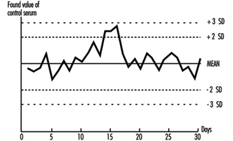
This approach can be adapted to a range of biological monitoring or biological effect monitoring assays. Batches of blood or urine samples can be prepared by addition of either the toxic material or the metabolite that is to be measured. Similarly, blood, serum, plasma, or urine can be aliquotted and stored deep-frozen or freeze-dried for measurement of enzymes or proteins. However, care has to be taken to avoid infective risk to the analyst from samples based on human blood.
Careful adherence to a well-defined protocol and to rules for acceptability is an essential first stage in a quality assurance programme. Any laboratory must be prepared to discuss its quality control and quality assessment performance with the health professionals using it and to investigate surprising or unusual findings.

External Quality Assessment
Once a laboratory has established that it can produce results with adequate precision, the next stage is to confirm the accuracy (“trueness”) of the measured values, that is, the relationship of the measurements made to the actual amount present. This is a difficult exercise for a laboratory to do on its own but can be achieved by taking part in a regular external quality assessment scheme. These have been an essential part of clinical chemistry practice for some time but have not been widely available for biological monitoring. The exception is blood lead analysis, where schemes have been available since the 1970s (e.g., Bullock, Smith and Whitehead 1986). Comparison of analytical results with those reported from other laboratories analysing samples from the same batch allows assessment of a laboratory’s performance compared with others, as well as a measure of its accuracy. Several national and international quality assessment schemes are available. Many of these schemes welcome new laboratories, as the validity of the mean of the results of an analyte from all the participating laboratories (taken as a measure of the actual concentration) increases with the number of participants. Schemes with many participants are also more able to analyse laboratory performance according to analytical method and thus advise on alternatives to methods with poor performance characteristics. In some countries, participation in such a scheme is an essential part of laboratory accreditation. Guidelines for external quality assessment scheme design and operation have been published by the WHO (1981).
In the absence of established external quality assessment schemes, accuracy may be checked using certified reference materials which are available on a commercial basis for a limited range of analytes. The advantages of samples circulated by external quality assessment schemes are that (1) the analyst does not have fore-knowledge of the result, (2) a range of concentrations is presented, and (3) as definitive analytical methods do not have to be employed, the materials involved are cheaper.

Pre-analytical Quality Control
Effort spent in attaining good laboratory accuracy and precision is wasted if the samples presented to the laboratory have not been taken at the correct time, if they have suffered contamination, have deteriorated during transport, or have been inadequately or incorrectly labelled. It is also bad professional practice to submit individuals to invasive sampling without taking adequate care of the sampled materials. Although sampling is often not under the direct control of the laboratory analyst, a full quality programme of biological monitoring must take these factors into account and the laboratory should ensure that syringes and sample containers provided are free from contamination, with clear instructions about sampling technique and sample storage and transport. The importance of the correct sampling time within the shift or working week and its dependence on the toxicokinetics of the sampled material are now recognized (ACGIH 1993; HSE 1992), and this information should be made available to the health professionals responsible for collecting the samples.

Post-analytical Quality Control
High-quality analytical results may be of little use to the individual or health professional if they are not communicated to the professional in an interpretable form and at the right time. Each biological monitoring laboratory should develop reporting procedures for alerting the health care professional submitting the samples to abnormal, unexpected, or puzzling results in time to allow appropriate action to be taken. Interpretation of laboratory results, especially changes in concentration between successive samples, often depends on knowledge of the precision of the assay. As part of total quality management from sample collection to return of results, health professionals should be given information concerning the biological monitoring laboratory’s precision and accuracy, as well as reference ranges and advisory and statutory limits, in order to help them in interpreting the results.

Click to return to top of page

Published in 27. Biological Monitoring

Monday, 28 February 2011 20:07

General Principles

Basic Concepts and Definitions

At the worksite, industrial hygiene methodologies can measure and control only airborne chemicals, while other aspects of the problem of possible harmful agents in the environment of workers, such as skin absorption, ingestion, and non-work-related exposure, remain undetected and therefore uncontrolled. Biological monitoring helps fill this gap.

Biological monitoring was defined in a 1980 seminar, jointly sponsored by the European Economic Community (EEC), National Institute for Occupational Safety and Health (NIOSH) and Occupational Safety and Health Association (OSHA) (Berlin, Yodaiken and Henman 1984) in Luxembourg as “the measurement and assessment of agents or their metabolites either in tissues, secreta, excreta, expired air or any combination of these to evaluate exposure and health risk compared to an appropriate reference”. Monitoring is a repetitive, regular and preventive activity designed to lead, if necessary, to corrective actions; it should not be confused with diagnostic procedures.

Biological monitoring is one of the three important tools in the prevention of diseases due to toxic agents in the general or occupational environment, the other two being environmental monitoring and health surveillance.

The sequence in the possible development of such disease may be schematically represented as follows: source-exposed chemical agent—internal dose—biochemical or cellular effect (reversible) —health effects—disease. The relationships among environmental, biological, and exposure monitoring, and health surveillance, are shown in figure 1.

Figure 1. The relationship between environmental, biological and exposure monitoring, and health surveillance

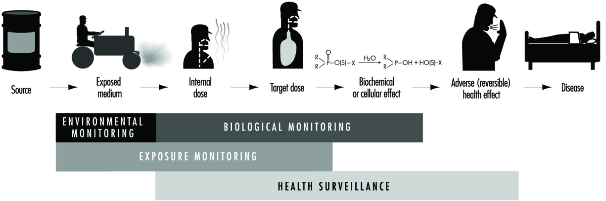
When a toxic substance (an industrial chemical, for example) is present in the environment, it contaminates air, water, food, or surfaces in contact with the skin; the amount of toxic agent in these media is evaluated via environmental monitoring.

As a result of absorption, distribution, metabolism, and excretion, a certain internal dose of the toxic agent (the net amount of a pollutant absorbed in or passed through the organism over a specific time interval) is effectively delivered to the body, and becomes detectable in body fluids. As a result of its interaction with a receptor in the critical organ (the organ which, under specific conditions of exposure, exhibits the first or the most important adverse effect), biochemical and cellular events occur. Both the internal dose and the elicited biochemical and cellular effects may be measured through biological monitoring.

Health surveillance was defined at the above-mentioned 1980 EEC/NIOSH/OSHA seminar as “the periodic medico-physiological examination of exposed workers with the objective of protecting health and preventing disease”.

Biological monitoring and health surveillance are parts of a continuum that can range from the measurement of agents or their metabolites in the body via evaluation of biochemical and cellular effects, to the detection of signs of early reversible impairment of the critical organ. The detection of established disease is outside the scope of these evaluations.

Goals of Biological Monitoring

Biological monitoring can be divided into (a) monitoring of exposure, and (b) monitoring of effect, for which indicators of internal dose and of effect are used respectively.

The purpose of biological monitoring of exposure is to assess health risk through the evaluation of internal dose, achieving an estimate of the biologically active body burden of the chemical in question. Its rationale is to ensure that worker exposure does not reach levels capable of eliciting adverse effects. An effect is termed “adverse” if there is an impairment of functional capacity, a decreased ability to compensate for additional stress, a decreased ability to maintain homeostasis (a stable state of equilibrium), or an enhanced susceptibility to other environmental influences.

Depending on the chemical and the analysed biological parameter, the term internal dose may have different meanings (Bernard and Lauwerys 1987). First, it may mean the amount of a chemical recently absorbed, for example, during a single workshift. A determination of the pollutant’s concentration in alveolar air or in the blood may be made during the workshift itself, or as late as the next day (samples of blood or alveolar air may be taken up to 16 hours after the end of the exposure period). Second, in the case that the chemical has a long biological half-life—for example, metals in the bloodstream—the internal dose could reflect the amount absorbed over a period of a few months.

Third, the term may also mean the amount of chemical stored. In this case it represents an indicator of accumulation which can provide an estimate of the concentration of the chemical in organs and/or tissues from which, once deposited, it is only slowly released. For example, measurements of DDT or PCB in blood could provide such an estimate.

Finally, an internal dose value may indicate the quantity of the chemical at the site where it exerts its effects, thus providing information about the biologically effective dose. One of the most promising and important uses of this capability, for example, is the determination of adducts formed by toxic chemicals with protein in haemoglobin or with DNA.

Biological monitoring of effects is aimed at identifying early and reversible alterations which develop in the critical organ, and which, at the same time, can identify individuals with signs of adverse health effects. In this sense, biological monitoring of effects represents the principal tool for the health surveillance of workers.

Principal Monitoring Methods

Biological monitoring of exposure is based on the determination of indicators of internal dose by measuring:

the amount of the chemical, to which the worker is exposed, in blood or urine (rarely in milk, saliva, or fat)
the amount of one or more metabolites of the chemical involved in the same body fluids
the concentration of volatile organic compounds (solvents) in alveolar air
the biologically effective dose of compounds which have formed adducts to DNA or other large molecules and which thus have a potential genotoxic effect.

Factors affecting the concentration of the chemical and its metabolites in blood or urine will be discussed below.

As far as the concentration in alveolar air is concerned, besides the level of environmental exposure, the most important factors involved are solubility and metabolism of the inhaled substance, alveolar ventilation, cardiac output, and length of exposure (Brugnone et al. 1980).

The use of DNA and haemoglobin adducts in monitoring human exposure to substances with carcinogenic potential is a very promising technique for measurement of low level exposures. (It should be noted, however, that not all chemicals that bind to macromolecules in the human organism are genotoxic, i.e., potentially carcinogenic.) Adduct formation is only one step in the complex process of carcinogenesis. Other cellular events, such as DNA repair promotion and progression undoubtedly modify the risk of developing a disease such as cancer. Thus, at the present time, the measurement of adducts should be seen as being confined only to monitoring exposure to chemicals. This is discussed more fully in the article “Genotoxic chemicals” later in this chapter.

Biological monitoring of effects is performed through the determination of indicators of effect, that is, those that can identify early and reversible alterations. This approach may provide an indirect estimate of the amount of chemical bound to the sites of action and offers the possibility of assessing functional alterations in the critical organ in an early phase.

Unfortunately, we can list only a few examples of the application of this approach, namely, (1) the inhibition of pseudocholinesterase by organophosphate insecticides, (2) the inhibition of d-aminolaevulinic acid dehydratase (ALA-D) by inorganic lead, and (3) the increased urinary excretion of d-glucaric acid and porphyrins in subjects exposed to chemicals inducing microsomal enzymes and/or to porphyrogenic agents (e.g., chlorinated hydrocarbons).

Advantages and Limitations of Biological Monitoring

For substances that exert their toxicity after entering the human organism, biological monitoring provides a more focused and targeted assessment of health risk than does environmental monitoring. A biological parameter reflecting the internal dose brings us one step closer to understanding systemic adverse effects than does any environmental measurement.

Biological monitoring offers numerous advantages over environmental monitoring and in particular permits assessment of:

exposure over an extended time period
exposure as a result of worker mobility in the working environment
absorption of a substance via various routes, including the skin
overall exposure as a result of different sources of pollution, both occupational and non-occupational
the quantity of a substance absorbed by the subject depending on factors other than the degree of exposure, such as the physical effort required by the job, ventilation, or climate
the quantity of a substance absorbed by a subject depending on individual factors that can influence the toxicokinetics of the toxic agent in the organism; for example, age, sex, genetic features, or functional state of the organs where the toxic substance undergoes biotransformation and elimination.

In spite of these advantages, biological monitoring still suffers today from considerable limitations, the most significant of which are the following:

The number of possible substances which can be monitored biologically is at present still rather small.
In the case of acute exposure, biological monitoring supplies useful information only for exposure to substances that are rapidly metabolized, for example, aromatic solvents.
The significance of biological indicators has not been clearly defined; for example, it is not always known whether the levels of a substance measured on biological material reflect current or cumulative exposure (e.g., urinary cadmium and mercury).
Generally, biological indicators of internal dose allow assessment of the degree of exposure, but do not furnish data that will measure the actual amount present in the critical organ
Often there is no knowledge of possible interference in the metabolism of the substances being monitored by other exogenous substances to which the organism is simultaneously exposed in the working and general environment.
There is not always sufficient knowledge on the relationships existing between the levels of environmental exposure and the levels of the biological indicators on the one hand, and between the levels of the biological indicators and possible health effects on the other.
The number of biological indicators for which biological exposure indices (BEIs) exist at present is rather limited. Follow-up information is needed to determine whether a substance, presently identified as not capable of causing an adverse effect, may at a later time be shown to be harmful.
A BEI usually represents a level of an agent that is most likely to be observed in a specimen collected from a healthy worker who has been exposed to the chemical to the same extent as a worker with an inhalation exposure to the TLV (threshold limit value) time-weighted average (TWA).

Information Required for the Development of Methods and Criteria for Selecting Biological Tests

Programming biological monitoring requires the following basic conditions:

knowledge of the metabolism of an exogenous substance in the human organism (toxicokinetics)
knowledge of the alterations that occur in the critical organ (toxicodynamics)
existence of indicators
existence of sufficiently accurate analytical methods
possibility of using readily obtainable biological samples on which the indicators can be measured
existence of dose-effect and dose-response relationships and knowledge of these relationships
predictive validity of the indicators.

In this context, the validity of a test is the degree to which the parameter under consideration predicts the situation as it really is (i.e., as more accurate measuring instruments would show it to be). Validity is determined by the combination of two properties: sensitivity and specificity. If a test possesses a high sensitivity, this means that it will give few false negatives; if it possesses high specificity, it will give few false positives (CEC 1985-1989).

Relationship between exposure, internal dose and effects

The study of the concentration of a substance in the working environment and the simultaneous determination of the indicators of dose and effect in exposed subjects allows information to be obtained on the relationship between occupational exposure and the concentration of the substance in biological samples, and between the latter and the early effects of exposure.

Knowledge of the relationships between the dose of a substance and the effect it produces is an essential requirement if a programme of biological monitoring is to be put into effect. The evaluation of this dose-effect relationship is based on the analysis of the degree of association existing between the indicator of dose and the indicator of effect and on the study of the quantitative variations of the indicator of effect with every variation of indicator of dose. (See also the chapter Toxicology, for further discussion of dose-related relationships).

With the study of the dose-effect relationship it is possible to identify the concentration of the toxic substance at which the indicator of effect exceeds the values currently considered not harmful. Furthermore, in this way it may also be possible to examine what the no-effect level might be.

Since not all the individuals of a group react in the same manner, it is necessary to examine the dose-response relationship, in other words, to study how the group responds to exposure by evaluating the appearance of the effect compared to the internal dose. The term response denotes the percentage of subjects in the group who show a specific quantitative variation of an effect indicator at each dose level.

Practical Applications of Biological Monitoring

The practical application of a biological monitoring programme requires information on (1) the behaviour of the indicators used in relation to exposure, especially those relating to degree, continuity and duration of exposure, (2) the time interval between end of exposure and measurement of the indicators, and (3) all physiological and pathological factors other than exposure that can alter the indicator levels.

In the following articles the behaviour of a number of biological indicators of dose and effect that are used for monitoring occupational exposure to substances widely used in industry will be presented. The practical usefulness and limits will be assessed for each substance, with particular emphasis on time of sampling and interfering factors. Such considerations will be helpful in establishing criteria for selecting a biological test.

Time of sampling

In selecting the time of sampling, the different kinetic aspects of the chemical must be kept in mind; in particular it is essential to know how the substance is absorbed via the lung, the gastrointestinal tract and the skin, subsequently distributed to the different compartments of the body, biotransformed, and finally eliminated. It is also important to know whether the chemical may accumulate in the body.

With respect to exposure to organic substances, the collection time of biological samples becomes all the more important in view of the different velocity of the metabolic processes involved and consequently the more or less rapid excretion of the absorbed dose.

Interfering Factors

Correct use of biological indicators requires a thorough knowledge of those factors which, although independent of exposure, may nevertheless affect the biological indicator levels. The following are the most important types of interfering factors (Alessio, Berlin and Foà 1987).

Physiological factors including diet, sex and age, for example, can affect results. Consumption of fish and crustaceans may increase the levels of urinary arsenic and blood mercury. In female subjects with the same lead blood levels as males, the erythrocyte protoporphyrin values are significantly higher compared to those of male subjects. The levels of urinary cadmium increase with age.

Among the personal habits that can distort indicator levels, smoking and alcohol consumption are particularly important. Smoking may cause direct absorption of substances naturally present in tobacco leaves (e.g., cadmium), or of pollutants present in the working environment that have been deposited on the cigarettes (e.g., lead), or of combustion products (e.g., carbon monoxide).

Alcohol consumption may influence biological indicator levels, since substances such as lead are naturally present in alcoholic beverages. Heavy drinkers, for example, show higher blood lead levels than control subjects. Ingestion of alcohol can interfere with the biotransformation and elimination of toxic industrial compounds: with a single dose, alcohol can inhibit the metabolism of many solvents, for example, trichloroethylene, xylene, styrene and toluene, because of their competition with ethyl alcohol for enzymes which are essential for the breakdown of both ethanol and solvents. Regular alcohol ingestion can also affect the metabolism of solvents in a totally different manner by accelerating solvent metabolism, presumably due to induction of the microsome oxidizing system. Since ethanol is the most important substance capable of inducing metabolic interference, it is advisable to determine indicators of exposure for solvents only on days when alcohol has not been consumed.

Less information is available on the possible effects of drugs on the levels of biological indicators. It has been demonstrated that aspirin can interfere with the biological transformation of xylene to methylhippuric acid, and phenylsalicylate, a drug widely used as an analgesic, can significantly increase the levels of urinary phenols. The consumption of aluminium-based antacid preparations can give rise to increased levels of aluminium in plasma and urine.

Marked differences have been observed in different ethnic groups in the metabolism of widely used solvents such as toluene, xylene, trichloroethylene, tetrachloroethylene, and methylchloroform.

Acquired pathological states can influence the levels of biological indicators. The critical organ can behave anomalously with respect to biological monitoring tests because of the specific action of the toxic agent as well as for other reasons. An example of situations of the first type is the behaviour of urinary cadmium levels: when tubular disease due to cadmium sets in, urinary excretion increases markedly and the levels of the test no longer reflect the degree of exposure. An example of the second type of situation is the increase in erythrocyte protoporphyrin levels observed in iron-deficient subjects who show no abnormal lead absorption.

Physiological changes in the biological media—urine, for example—on which determinations of the biological indicators are based, can influence the test values. For practical purposes, only spot urinary samples can be obtained from individuals during work, and the varying density of these samples means that the levels of the indicator can fluctuate widely in the course of a single day.

In order to overcome this difficulty, it is advisable to eliminate over-diluted or over-concentrated samples according to selected specific gravity or creatinine values. In particular, urine with a specific gravity below 1010 or higher than 1030 or with a creatinine concentration lower than 0.5 g/l or greater than 3.0 g/l should be discarded. Several authors also suggest adjusting the values of the indicators according to specific gravity or expressing the values according to urinary creatinine content.

Pathological changes in the biological media can also considerably influence the values of the biological indicators. For example, in anaemic subjects exposed to metals (mercury, cadmium, lead, etc.) the blood levels of the metal may be lower than would be expected on the basis of exposure; this is due to the low level of red blood cells that transport the toxic metal in the blood circulation.

Therefore, when determinations of toxic substances or metabolites bound to red blood cells are made on whole blood, it is always advisable to determine the haematocrit, which gives a measure of the percentage of blood cells in whole blood.

Multiple exposure to toxic substances present in the workplace

In the case of combined exposure to more than one toxic substance present at the workplace, metabolic interferences may occur that can alter the behaviour of the biological indicators and thus create serious problems in interpretation. In human studies, interferences have been demonstrated, for example, in combined exposure to toluene and xylene, xylene and ethylbenzene, toluene and benzene, hexane and methyl ethyl ketone, tetrachloroethylene and trichloroethylene.

In particular, it should be noted that when biotransformation of a solvent is inhibited, the urinary excretion of its metabolite is reduced (possible underestimation of risk) whereas the levels of the solvent in blood and expired air increase (possible overestimation of risk).

Thus, in situations in which it is possible to measure simultaneously the substances and their metabolites in order to interpret the degree of inhibitory interference, it would be useful to check whether the levels of the urinary metabolites are lower than expected and at the same time whether the concentration of the solvents in blood and/or expired air is higher.

Metabolic interferences have been described for exposures where the single substances are present in levels close to and sometimes below the currently accepted limit values. Interferences, however, do not usually occur when exposure to each substance present in the workplace is low.

Practical Use of Biological Indicators

Biological indicators can be used for various purposes in occupational health practice, in particular for (1) periodic control of individual workers, (2) analysis of the exposure of a group of workers, and (3) epidemiological assessments. The tests used should possess the features of precision, accuracy, good sensitivity, and specificity in order to minimize the possible number of false classifications.

Reference values and reference groups

A reference value is the level of a biological indicator in the general population not occupationally exposed to the toxic substance under study. It is necessary to refer to these values in order to compare the data obtained through biological monitoring programmes in a population which is presumed to be exposed. Reference values should not be confused with limit values, which generally are the legal limits or guidelines for occupational and environmental exposure (Alessio et al. 1992).

When it is necessary to compare the results of group analyses, the distribution of the values in the reference group and in the group under study must be known because only then can a statistical comparison be made. In these cases, it is essential to attempt to match the general population (reference group) with the exposed group for similar characteristics such as, sex, age, lifestyle and eating habits.

To obtain reliable reference values one must make sure that the subjects making up the reference group have never been exposed to the toxic substances, either occupationally or due to particular conditions of environmental pollution.

In assessing exposure to toxic substances one must be careful not to include subjects who, although not directly exposed to the toxic substance in question, work in the same workplace, since if these subjects are, in fact, indirectly exposed, the exposure of the group may be in consequence underestimated.

Another practice to avoid, although it is still widespread, is the use for reference purposes of values reported in the literature that are derived from case lists from other countries and may often have been collected in regions where different environmental pollution situations exist.

Periodic monitoring of individual workers

Periodic monitoring of individual workers is mandatory when the levels of the toxic substance in the atmosphere of the working environment approach the limit value. Where possible, it is advisable to simultaneously check an indicator of exposure and an indicator of effect. The data thus obtained should be compared with the reference values and the limit values suggested for the substance under study (ACGIH 1993).

Analysis of a group of workers

Analysis of a group becomes mandatory when the results of the biological indicators used can be markedly influenced by factors independent of exposure (diet, concentration or dilution of urine, etc.) and for which a wide range of “normal” values exists.

In order to ensure that the group study will furnish useful results, the group must be sufficiently numerous and homogeneous as regards exposure, sex, and, in the case of some toxic agents, work seniority. The more the exposure levels are constant over time, the more reliable the data will be. An investigation carried out in a workplace where the workers frequently change department or job will have little value. For a correct assessment of a group study it is not sufficient to express the data only as mean values and range. The frequency distribution of the values of the biological indicator in question must also be taken into account.

Epidemiological assessments

Data obtained from biological monitoring of groups of workers can also be used in cross-sectional or prospective epidemiological studies.

Cross-sectional studies can be used to compare the situations existing in different departments of the factory or in different industries in order to set up risk maps for manufacturing processes. A difficulty that may be encountered in this type of application depends on the fact that inter-laboratory quality controls are not yet sufficiently widespread; thus it cannot be guaranteed that different laboratories will produce comparable results.

Prospective studies serve to assess the behaviour over time of the exposure levels so as to check, for example, the efficacy of environmental improvements or to correlate the behaviour of biological indicators over the years with the health status of the subjects being monitored. The results of such long-term studies are very useful in solving problems involving changes over time. At present, biological monitoring is mainly used as a suitable procedure for assessing whether current exposure is judged to be “safe,” but it is as yet not valid for assessing situations over time. A given level of exposure considered safe today may no longer be regarded as such at some point in the future.

Ethical Aspects

Some ethical considerations arise in connection with the use of biological monitoring as a tool to assess potential toxicity. One goal of such monitoring is to assemble enough information to decide what level of any given effect constitutes an undesirable effect; in the absence of sufficient data, any perturbation will be considered undesirable. The regulatory and legal implications of this type of information need to be evaluated. Therefore, we should seek societal discussion and consensus as to the ways in which biological indicators should best be used. In other words, education is required of workers, employers, communities and regulatory authorities as to the meaning of the results obtained by biological monitoring so that no one is either unduly alarmed or complacent.

There must be appropriate communication with the individual upon whom the test has been performed concerning the results and their interpretation. Further, whether or not the use of some indicators is experimental should be clearly conveyed to all participants.

The International Code of Ethics for Occupational Health Professionals, issued by the International Commission on Occupational Health in 1992, stated that “biological tests and other investigations must be chosen from the point of view of their validity for protection of the health of the worker concerned, with due regard to their sensitivity, their specificity and their predictive value”. Use must not be made of tests “which are not reliable or which do not have a sufficient predictive value in relation to the requirements of the work assignment”. (See the chapter Ethical Issues for further discussion and the text of the Code.)

Trends in Regulation and Application

Biological monitoring can be carried out for only a limited number of environmental pollutants on account of the limited availability of appropriate reference data. This imposes important limitations on the use of biological monitoring in evaluating exposure.

The World Health Organization (WHO), for example, has proposed health-based reference values for lead, mercury, and cadmium only. These values are defined as levels in blood and urine not linked to any detectable adverse effect.The American Conference of Governmental Industrial Hygienists (ACGIH) has established biological exposure indices (BEIs) for about 26 compounds; BEIs are defined as “values for determinants which are indicators of the degree of integrated exposure to industrial chemicals” (ACGIH 1995).

Back

Published in 27. Biological Monitoring

Monday, 28 February 2011 19:43

Prevention and Standards

Hazards and Preventive Measures at Electrical Facilities

The many components making up electrical installations exhibit varying degrees of robustness. Regardless of their inherent fragility, however, they must all operate reliably under rigorous conditions. Unfortunately, even under the best circumstances, electrical equipment is subject to failures that may result in human injury or material damage.

Safe operation of electrical installations is the result of good initial design, not the mere retrofitting of safety systems. This is a corollary of the fact that while current flows at the speed of light, all electromechanical and electronic systems exhibit reaction latencies, caused primarily by thermal inertia, mechanical inertia and maintenance conditions. These latencies, whatever their origins, are sufficiently lengthy to allow humans to be injured and equipment damaged (Lee, Capelli-Schellpfeffer and Kelly 1994; Lee, Cravalho and Burke 1992; Kane and Sternheim 1978).

It is essential that equipment be installed and maintained by qualified personnel. Technical measures, it should be emphasized, are necessary both to ensure the safe operation of installations and to protect humans and equipment.

Introduction to electrical hazards

Proper operation of electrical installations requires that machinery, equipment, and electrical circuits and lines be protected from hazards caused by both internal (i.e., arising within the installation) and external factors (Andreoni and Castagna 1983).

Internal causes include:

overvoltages

short circuits

modification of the current’s wave-form

induction

interference

overcurrents

corrosion, leading to electrical current leakages to ground

heating of conducting and insulating materials, which may result in operator burns, emissions of toxic gases, component fires and, in flammable atmospheres, explosions

leaks of insulating fluids, such as oil

generation of hydrogen or other gases which may lead to the formation of explosive mixtures.

Each hazard-equipment combination requires specific protective measures, some of which are mandated by law or internal technical regulations. Manufacturers have a responsibility to be aware of specific technical strategies capable of reducing risks.

External causes include:

mechanical factors (falls, bumps, vibration)

physical and chemical factors (natural or artificial radiation, extreme temperatures, oils, corrosive liquids, humidity)

wind, ice, lightning

vegetation (trees and roots, both dry and wet)

animals (in both urban and rural settings); these may damage the power-line insulation, and so cause short circuits or false contacts

and, last but not least,

adults and children who are careless, reckless or ignorant of risks and operating procedures.

Other external causes include electromagnetic interference by sources such as high-voltage lines, radio receivers, welding machines (capable of generating transient overvoltages) and solenoids.

The most frequently encountered causes of problems arise from malfunctioning or non-standard:

mechanical, thermal or chemical protective equipment
ventilation systems, machine cooling systems, equipment, lines or circuits
coordination of insulators used in different parts of the plant
coordination of fuses and automatic circuit-breakers.

A single fuse or automatic circuit-breaker is incapable of providing adequate protection against overcurrent on two different circuits. Fuses or automatic circuit breakers can provide protection against phase-neutral failures, but protection against phase-ground failures requires automatic residual-current circuit-breakers.

use of voltage relays and dischargers to coordinate protective systems
sensors and mechanical or electrical components in the installation’s protective systems
separation of circuits at different voltages (adequate air gaps must be maintained between conductors; connections should be insulated; transformers should be equipped with grounded shields and suitable protection against overvoltage, and have fully segregated primary and secondary coils)
colour codes or other suitable provisions to avoid misidentification of wires
mistaking the active phase for a neutral conductor results in electrification of the equipment’s external metallic components
protective equipment against electromagnetic interference.

These are particularly important for instrumentation and lines used for data transmission or the exchange of protection and/or controlling signals. Adequate gaps must be maintained between lines, or filters and shields used. Fibre-optic cables are sometimes used for the most critical cases.

The risk associated with electrical installations increases when the equipment is subjected to severe operating conditions, most commonly as a result of electrical hazards in humid or wet environments.

The thin liquid conductive layers that form on metallic and insulating surfaces in humid or wet environments create new, irregular and dangerous current pathways. Water infiltration reduces the efficiency of insulation, and, should water penetrate the insulation, it can cause current leakages and short circuits. These effects not only damage electrical installations but greatly increase human risks. This fact justifies the need for special standards for work in harsh environments such as open-air sites, agricultural installations, construction sites, bathrooms, mines and cellars, and some industrial settings.

Equipment providing protection against rain, side-splashes or full immersion is available. Ideally, the equipment should be enclosed, insulated and corrosion proof. Metallic enclosures must be grounded. The mechanism of failure in these wet environments is the same as that observed in humid atmospheres, but the effects may be more severe.

Electrical hazards in dusty atmospheres

Fine dusts that enter machines and electrical equipment cause abrasion, particularly of mobile parts. Conducting dusts may also cause short circuits, while insulating dusts may interrupt current flow and increase contact resistance. Accumulations of fine or coarse dusts around equipment cases are potential humidity and water reservoirs. Dry dust is a thermal insulator, reducing heat dispersion and increasing local temperature; this may damage electrical circuits and cause fires or explosions.

Water- and explosion-proof systems must be installed in industrial or agricultural sites where dusty processes are carried out.

Electrical hazards in explosive atmospheres or at sites containing explosive materials

Explosions, including those of atmospheres containing explosive gases and dusts, may be triggered by opening and closing live electrical circuits, or by any other transient process capable of generating sparks of sufficient energy.

This hazard is present in sites such as:

mines and underground sites where gases, especially methane, may accumulate
chemical industries
lead-battery storage rooms, where hydrogen may accumulate
the food industry, where natural organic powders may be generated
the synthetic materials industry
metallurgy, especially that involving aluminium and magnesium.

Where this hazard is present, the number of electrical circuits and equipment should be minimized—for example, by removing electrical motors and transformers or replacing them with pneumatic equipment. Electrical equipment which cannot be removed must be enclosed, to avoid any contact of flammable gases and dusts with sparks, and a positive-pressure inert-gas atmosphere maintained within the enclosure. Explosion-proof enclosures and fireproof electrical cables must be used where there is the possibility of explosion. A full range of explosion-proof equipment has been developed for some high-risk industries (e.g., the oil and chemical industries).

Because of the high cost of explosion-proof equipment, plants are commonly divided into electrical hazard zones. In this approach, special equipment is used in high-risk zones, while a certain amount of risk is accepted in others. Various industry-specific criteria and technical solutions have been developed; these usually involve some combination of grounding, component segregation and the installation of zoning barriers.

Equipotential Bonding

If all the conductors, including the earth, that can be touched simultaneously were at the same potential, there would be no danger to humans. Equipotential bonding systems are an attempt to achieve this ideal condition (Andreoni and Castagna 1983; Lee, Cravalho and Burke 1992).

In equipotential bonding, every exposed conductor of non-transmission electrical equipment and every accessible extraneous conductor in the same site are connected to a protective grounded conductor. It should be recalled that while the conductors of non-transmission equipment are dead during normal operation, they may become live following insulation failure. By decreasing the contact voltage, equipotential bonding prevents metallic components from reaching voltages that are hazardous to both humans and equipment.

In practice, it may prove necessary to connect the same machine to the equipotential bonding grid at more than one point. Areas of poor contact, due, for example, to the presence of insulators such as lubricants and paint, should be carefully identified. Similarly, it is good practice to connect all the local and external service piping (e.g., water, gas and heating) to the equipotential bonding grid.

Grounding

In most cases, it is necessary to minimize the voltage drop between the installation’s conductors and the earth. This is accomplished by connecting the conductors to a grounded protective conductor.

There are two types of ground connections:

functional grounds—for example, grounding the neutral conductor of a three-phase system, or the midpoint of a transformer’s secondary coil
protective grounds—for example, grounding every conductor on a piece of equipment. The object of this type of grounding is to minimize conductor voltages by creating a preferential path for fault currents, especially those currents likely to affect humans.

Under normal operating conditions, no current flows through ground connections. In the event of accidental activation of the circuit, however, the current flow through the low-resistance grounding connection is high enough to melt the fuse or the ungrounded conductors.

The maximum fault voltage in equipotential grids allowed by most standards is 50 V for dry environments, 25 V for wet or humid environments and 12 V for medical laboratories and other high-risk environments. Although these values are only guidelines, the necessity of ensuring adequate grounding in workplaces, public spaces and especially residences, should be emphasized.

The efficiency of grounding depends primarily on the existence of high and stable ground leakage currents, but also on adequate galvanic coupling of the equipotential grid, and the diameter of the conductors leading to the grid. Because of the importance of ground leakage, it must be evaluated with great accuracy.

Ground connections must be as reliable as equipotential grids, and their proper operation must be verified on a regular basis.

As the earth resistance increases, the potential of both the grounding conductor and the earth around the conductor approaches that of the electrical circuit; in the case of the earth around the conductor, the potential generated is inversely proportional to the distance from the conductor. In order to avoid dangerous step voltages, ground conductors must be properly shielded and set in the ground at adequate depths.

As an alternative to equipment grounding, standards allow for the use of double-insulated equipment. This equipment, recommended for use in residential settings, minimizes the chance of insulation failure by providing two separate insulation systems. Double-insulated equipment cannot be relied upon to adequately protect against interface failures such as those associated with loose but live plugs, since some countries’ plug and wall-socket standards do not address the use of such plugs.

Circuit-breakers

The surest method of reducing electrical hazards to humans and equipment is to minimize the duration of the fault current and voltage increase, ideally before the electrical energy has even begun to increase. Protective systems in electrical equipment usually incorporate three relays: a residual-current relay to protect against failure towards ground, a magnetic relay and a thermal relay to protect against overloads and short circuits.

In residual-current circuit-breakers, the conductors in the circuit are wound around a ring which detects the vector sum of the currents entering and exiting the equipment to be protected. The vector sum is equal to zero during normal operation, but equals the leakage current in cases of failure. When the leakage current reaches the breaker’s threshold, the breaker is tripped. Residual-current circuit-breakers can be tripped by currents as low as 30 mA, with latencies as low as 30 ms.

The maximum current that can be safely carried by a conductor is a function of its cross-sectional area, insulation and installation. Overheating will result if the maximum safe load is exceeded or if heat dissipation is limited. Overcurrent devices such as fuses and magneto-thermal circuit-breakers automatically break the circuit if excessive current flow, ground faults, overloading or short circuits occur. Overcurrent devices should interrupt the current flow when it exceeds the conductor’s capacity.

Selection of protective equipment capable of protecting both personnel and equipment is one of the most important issues in the management of electrical installations and must take into account not only the current-carrying capacity of conductors but also the characteristics of the circuits and the equipment connected to them.

Special high-capacity fuses or circuit-breakers must be used on circuits carrying very high current loads.

Fuses

Several types of fuse are available, each designed for a specific application. Use of the wrong type of fuse or of a fuse of the wrong capacity may cause injury and damage equipment. Overfusing frequently results in overheated wiring or equipment, which in turn may cause fires.

Before replacing fuses, lock out, tag and test the circuit, to verify that the circuit is dead. Testing can save lives. Next, identify the cause of any short circuits or overloads, and replace blown fuses with fuses of the same type and capacity. Never insert fuses in a live circuit.

Circuit-breakers

Although circuit-breakers have long been used in high-voltage circuits with large current capacities, they are increasingly used in many other kinds of circuits. Many types are available, offering a choice of immediate and delayed onset and manual or automatic operation.

Circuit-breakers fall into two general categories: thermal and magnetic.

Thermal circuit-breakers react solely to a rise of temperature. Variations in the circuit-breaker’s ambient temperature will therefore affect the point at which the breaker is tripped.

Magnetic circuit-breakers, on the other hand, react solely to the amount of current passing through the circuit. This type of breaker is preferable where wide temperature fluctuations would require overrating the circuit-breaker, or where the breaker is frequently tripped.

In the case of contact with lines carrying high current loads, protective circuits cannot prevent personal injury or equipment damage, as they are designed only to protect power-lines and systems from excess current flow caused by faults.

Because of the resistance of the contact with the earth, the current passing through an object simultaneously contacting the line and the earth will usually be less than the tripping current. Fault currents flowing through humans may be further reduced by body resistance to the point where they do not trip the breaker, and are therefore extremely dangerous. It is virtually impossible to design a power system that would prevent injury or damage to any object that faults the power lines while remaining a useful energy transmission system, as the trip thresholds for the relevant circuit protection devices are well above the human hazard level.

Standards and Regulations

The framework of international standards and regulations is illustrated in figure 1 (Winckler 1994). The rows correspond to the geographic scope of the standards, either worldwide (international), continental (regional) or national, while the columns correspond to the standards’ fields of application. The IEC and the International Organization for Standardization (ISO) both share an umbrella structure, the Joint Presidents Coordinating Group (JPCG); the European equivalent is the Joint Presidents Group (JPG).

Figure 1. The framework of international standards and regulations

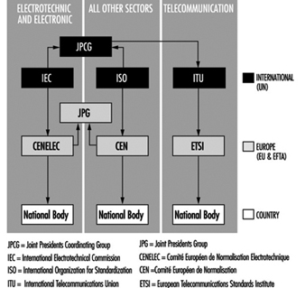
Each standardization body holds regular international meetings. The composition of the various bodies reflects the development of standardization.

The Comité européen de normalisation électrotechnique (CENELEC) was created by the electrical engineering committees of the countries signing the 1957 Rome Treaty establishing the European Economic Community. The six founding members were later joined by the members of the European Free Trade Association (EFTA), and CENELEC in its present form dates from 13 February, 1972.

In contrast to the International Electrotechnical Commission (IEC), CENELEC focuses on the implementation of international standards in member countries rather than on the creation of new standards. It is particularly important to recall that while the adoption of IEC standards by member countries is voluntary, adoption of CENELEC standards and regulations is obligatory in the European Union. Over 90% of CENELEC standards are derived from IEC standards, and over 70% of them are identical. CENELEC’s influence has also attracted the interest of Eastern European countries, most of which became affiliated members in 1991.

The International Association for Testing and Materials, the forerunner of the ISO, as it is known today, was founded in 1886 and was active until The First World War, after which it ceased to function as an international association. Some national organizations, like the American Society for Testing and Materials (ASTM), survived. In 1926, the International Standards Association (ISA) was founded in New York and was active until The Second World War. The ISA was replaced in 1946 by the ISO, which is responsible for all fields except electrical engineering and telecommunications. The Comité européen de normalisation (CEN) is the European equivalent of the ISO and has the same function as CENELEC, although only 40% of CEN standards are derived from ISO standards.

The current wave of international economic consolidation creates a need for common technical databases in the field of standardization. This process is presently under way in several parts of the world, and it is likely that new standardization bodies will evolve outside of Europe. CANENA is a regional standardization body created by the North American Free Trade Agreement (NAFTA) countries (Canada, Mexico and the United States). Wiring of premises in the US is governed by the National Electrical Code, ANSI/NFPA 70-1996. This Code is also in use in several other countries in North and South America. It provides installation requirements for premises wiring installations beyond the point of connection to the electric utility system. It covers installation of electric conductors and equipment within or on public and private buildings, including mobil homes, recreational vehicles, and floating buildings, stock yards, carnivals, parking and other lots, and industrial substations. It does not cover installations in ships or watercraft other than floating buildings—railway rolling stop, aircraft, or automotive vehicles. The National Electric Code also does not apply to other areas that are normally regulated by the National Electrical Safety Code, such as installations of communications utility equipment and electric utility installations.

European and American Standards for the Operation of Electrical Installations

The European Standard EN 50110-1, Operation of Electrical Installations (1994a) prepared by CENELEC Task Force 63-3, is the basic document that applies to the operation of and work activities on, with or near electrical installations. The standard sets the minimum requirements for all CENELEC countries; additional national standards are described in separate subparts of the standard (EN 50110-2).

The standard applies to installations designed for the generation, transmission, conversion, distribution and use of electrical power, and operating at commonly encountered voltage levels. Although typical installations operate at low voltages, the standard also applies to extra-low and high-voltage installations. Installations may be either permanent and fixed (e.g., distribution installations in factories or office complexes) or mobile.

Safe operation and maintenance procedures for work on or near electrical installations are set out in the standard. Applicable work activities include non-electrical work such as construction near overhead lines or underground cables, in addition to all types of electrical work. Certain electrical installations, such as those on board aircraft and ships, are not subject to the standard.

The equivalent standard in the United States is the National Electrical Safety Code (NESC), American National Standards Institute (1990). The NESC applies to utility facilities and functions from the point of generation of electricity and communication signals, through the transmission grid, to the point of delivery to a customer’s facilities. Certain installations, including those in mines and ships, are not subject to the NESC. NESC guidelines are designed to ensure the safety of workers engaged in the installation, operation or maintenance of electric supply and communication lines and associated equipment. These guidelines constitute the minimum acceptable standard for occupational and public safety under the specified conditions. The code is not intended as a design specification or an instruction manual. Formally, the NESC must be regarded as a national safety code applicable to the United States.

The extensive rules of both the European and American standards provide for the safe performance of work on electrical installations.

The European Standard (1994a)

Definitions

The standard provides definitions only for the most common terms; further information is available in the International Electrotechnical Commission (1979). For the purposes of this standard, electrical installation refers to all equipment involved in the generation, transmission, conversion, distribution and use of electrical energy. This includes all energy sources, including batteries and capacitors (ENEL 1994; EDF-GDF 1991).

Basic principles

Safe operation: The basic principle of safe work on, with or near an electrical installation is the need to assess the electrical risk before commencing work.

Personnel: The best rules and procedures for work on, with or near electrical installations are of no value if workers are not thoroughly conversant with them and do not comply strictly with them. All personnel involved in work on, with or near an electrical installation shall be instructed in the safety requirements, safety rules and company policies applicable to their work. Where the work is long or complex, this instruction shall be repeated. Workers shall be required to comply with these requirements, rules and instructions.

Organization: Each electrical installation shall be placed under the responsibility of the designated person in control of the electrical installation. In cases of undertakings involving more than one installation, it is essential that the designated persons in control of each installation cooperate with each other.

Each work activity shall be the responsibility of the designated person in control of the work. Where the work comprises sub-tasks, persons responsible for the safety of each sub-task will be designated, each reporting to the coordinator. The same person can act as the designated person in control of the work and the designated person in control of the electrical installation.

Communication: This includes all means of information transmission between persons, i.e., spoken word (including telephones, radio and speech), writing (including fax) and visual means (including instrument panels, video, signals and lights).

Formal notification of all information necessary for the safe operation of the electrical installation, e.g., network arrangements, switchgear status and the position of safety devices, shall be given.

Worksite: Adequate working space, access and lighting shall be provided at electrical installations on, with or near which any work is to be carried out.

Tools, equipment and procedures: Tools, equipment and procedures shall comply with the requirements of relevant European, national and international standards, where these exist.

Drawings and reports: The installation’s drawings and reports shall be up to date and readily available.

Signage: Adequate signage drawing attention to specific hazards shall be displayed as needed when the installation is operating and during any work.

Standard operating procedures

Operating activities: Operating activities are designed to change the electrical state of an electrical installation. There are two types:

operations intended to modify the electrical state of an electrical installation, e.g., in order to use equipment, connect, disconnect, start or stop an installation or section of an installation to carry out work. These activities may be carried out locally or by remote control.
disconnecting before or reconnecting after dead-working, to be carried out by qualified or trained workers.

Functional checks: This includes measurement, testing and inspection procedures.

Measurement is defined as the entire range of activities used to collect physical data in electrical installations. Measurement shall be carried out by qualified professionals.

Testing includes all activities designed to verify the operation or electrical, mechanical or thermal condition of an electrical installation. Testing shall be carried out by qualified workers.

Inspection is verification that an electrical installation conforms to applicable specified technical and safety regulations.

Work procedures

General: The designated person in control of the electrical installation and the designated person in control of the work shall both ensure that workers receive specific and detailed instructions before starting the work, and on its completion.

Before the start of work, the designated person in control of the work shall notify the designated person in control of the electrical installation of the nature, site and consequences to the electrical installation of the intended work. This notification shall be given preferably in writing, especially when the work is complex.

Work activities can be divided into three categories: dead-working, live-working and work in the vicinity of live installations. Measures designed to protect against electrical shocks, short circuits and arcing have been developed for each type of work.

Induction: The following precautions shall be taken when working on electrical lines subject to current induction:

grounding at appropriate intervals; this reduces the potential between conductors and earth to a safe level
equipotential bonding of the worksite; this prevents workers from introducing themselves into the induction loop.

Weather conditions: When lightning is seen or thunder heard, no work shall be started or continued on outdoor installations or on indoor installations directly connected to overhead lines.

Dead-working

The following basic work practices will ensure that the electrical installations at the worksite remain dead for the duration of the work. Unless there are clear contraindications, the practices should be applied in the order listed.

Complete disconnection: The section of the installation in which the work is to be carried out shall be isolated from all sources of current supply, and secured against reconnection.

Securing against reconnection: All circuit-breaking devices used to isolate the electrical installation for the work shall be locked out, preferably by locking the operating mechanism.

Verification that the installation is dead: The absence of current shall be verified at all poles of the electrical installation at or as near as practicable to the worksite.

Grounding and short-circuiting: At all high- and some low-voltage worksites, all parts to be worked on shall be grounded and short-circuited after they have been disconnected. Grounding and short-circuiting systems shall be connected to the earth first; the components to be grounded must be connected to the system only after it has been earthed. As far as practical, the grounding and short-circuiting systems shall be visible from the worksite. Low- and high-voltage installations have their own specific requirements. At these types of installation, all sides of the worksites and all conductors entering the site must be grounded and short-circuited.

Protecting against adjacent live parts: Additional protective measures are necessary if parts of an electrical installation in the vicinity of the worksite cannot be made dead. Workers shall not commence work before receiving permission to do so from the designated person in control of the work, who in turn must receive authorization from the designated person in control of the electrical installation. Once the work has been completed, workers shall leave the worksite, tools and equipment shall be stored, and grounding and short-circuiting systems removed. The designated person in control of the work shall then notify the designated person in control of the electrical installation that the installation is available for reconnection.

Live-working

General: Live-working is work carried out within a zone in which there is current flow. Guidance for the dimensions of the live-working zone can be found in standard EN 50179. Protective measures designed to prevent electric shocks, arcing and short circuits shall be applied.

Training and qualification: Specific training programmes shall be established to develop and maintain the ability of qualified or trained workers to perform live-working. After completing the programme, workers will receive a qualification rating and authorization to perform specific live-work on specific voltages.

Maintenance of qualifications: The ability to carry out live-working shall be maintained by either practice or new training.

Work techniques: Currently, there are three recognized techniques, distinguished by their applicability to different types of live parts and the equipment required to prevent electric shocks, arcing and short circuits:

hot-stick working
insulating-glove working
bare-hand working.

Each technique requires different preparation, equipment and tools, and selection of the most appropriate technique will depend on the characteristics of the work in question.

Tools and equipment: The characteristics, storage, maintenance, transportation and inspection of tools, equipment and systems shall be specified.

Weather conditions: Restrictions apply to live-working in adverse weather conditions, since insulating properties, visibility and worker mobility are all reduced.

Work organization: The work shall be adequately prepared; written preparation shall be submitted in advance for complex work. The installation in general, and the section where the work is to be carried out in particular, shall be maintained in a condition consistent with the preparation required. The designated person in control of the work shall inform the designated person in control of the electrical installation of the nature of the work, the site in the installation at which the work will be performed, and the estimated duration of the work. Before work begins, workers shall have the nature of the work, the relevant safety measures, the role of each worker, and the tools and equipment to be used explained to them.

Specific practices exist for extra-low-voltage, low-voltage, and high-voltage installations.

Work in the vicinity of live parts

General: Work in the vicinity of live parts with nominal voltages above 50 VAC or 120 VDC shall be performed only when safety measures have been applied to ensure that live parts cannot be touched or that the live zone cannot be entered. Screens, barriers, enclosures or insulating coverings may be used for this purpose.

Before the work starts, the designated person in control of the work shall instruct the workers, particularly those unfamiliar with work in the vicinity of live parts, on the safety distances to be observed on the worksite, the principal safety practices to follow, and the need for behaviour that ensures the safety of the entire work crew. Worksite boundaries shall be precisely defined and marked and attention drawn to unusual working conditions. This information shall be repeated as needed, particularly after changes in working conditions.

Workers shall ensure that no part of their body nor any object enters the live zone. Particular care shall be taken when handling long objects, for example, tools, cable ends, pipes and ladders.

Protection by screens, barriers, enclosures or insulating coverings: The selection and installation of these protective devices shall ensure sufficient protection against predictable electrical and mechanical stressors. The equipment shall be suitably maintained and kept secured during the work.

Maintenance

General: The purpose of maintenance is to maintain the electrical installation in the required condition. Maintenance may be preventive (i.e., carried out on a regular basis to prevent breakdowns and keep equipment in working order) or corrective (i.e., carried out to replace defective parts).

Maintenance work can be divided into two risk categories:

work involving the risk of electrical shock, where procedures applicable to live-working and work in the vicinity of live parts must be followed
work where equipment design allows some maintenance work to be performed in the absence of full live-working procedures

Personnel: Personnel who are to carry out the work shall be adequately qualified or trained and shall be provided with appropriate measuring and testing tools and devices.

Repair work: Repair work consists of the following steps: fault location; fault rectification and/or replacement of components; recommissioning of the repaired section of the installation. Each of these steps may require specific procedures.

Replacement work: In general, fuse replacement in high-voltage installations shall be performed as dead-work. Fuse replacement shall be performed by qualified workers following appropriate work procedures. The replacement of lamps and removable parts such as starters shall be carried out as dead-work. In high-voltage installations, repair procedures shall also apply to replacement work.

Training of Personnel about Electrical Hazards

Effective work organization and safety training is a key element in every successful organization, prevention programme and occupational health and safety programme. Workers must have proper training to do their jobs safely and efficiently.

The responsibility for implementing employee training rests with management. Management must recognize that employees must perform at a certain level before the organization can achieve its objectives. In order to achieve these levels, worker training policies and, by extension, concrete training programmes must be established. Programmes should include training and qualification phases.

Live-working programmes should include the following elements:

Training: In some countries, programmes and training facilities must be formally approved by a live-working committee or similar body. Programmes are based primarily on practical experience, complemented by technical instruction. Training takes the form of practical work on indoor or outdoor model installations similar to those on which actual work is to be performed.

Qualifications: Live-working procedures are very demanding, and it is essential to use the right person at the right place. This is most easily achieved if qualified personnel of different skill levels are available. The designated person in control of the work should be a qualified worker. Where supervision is necessary, it too should be carried out by a qualified person. Workers should work only on installations whose voltage and complexity corresponds to their level of qualification or training. In some countries, qualification is regulated by national standards.

Finally, workers should be instructed and trained in essential life-saving techniques. The reader is referred to the chapter on first-aid for further information.

Back

Published in 40. Electricity

Monday, 28 February 2011 19:25

Static Electricity

All materials differ in the degree to which electric charges can pass through them. Conductors allow charges to flow, while insulators hinder the motion of charges. Electrostatics is the field devoted to studying charges, or charged bodies at rest. Static electricity results when electric charges which do not move are built up on objects. If the charges flow, then a current results and the electricity is no longer static. The current that results from moving charges is commonly referred to by laypeople as electricity, and is discussed in the other articles in this chapter. Static electrification is the term used to designate any process resulting in the separation of positive and negative electrical charges. Conduction is measured with a property called conductance, while an insulator is characterized by its resistivity. Charge separation which leads to electrification can occur as the result of mechanical processes—for example, contact between objects and friction, or the collision of two surfaces. The surfaces can be two solids or a solid and a liquid. The mechanical process can, less commonly, be the rupture or separation of solid or liquid surfaces. This article focuses on contact and friction.

Electrification Processes

The phenomenon of generation of static electricity by friction (triboelectrification) has been known for thousands of years. Contact between two materials is sufficient to induce electrification. Friction is simply a type of interaction which increases the area of contact and generates heat—friction is the general term to describe the movement of two objects in contact; the pressure exerted, its shear velocity and the heat generated are the prime determinants of the charge generated by friction. Sometimes friction will lead to the tearing away of solid particles as well.

When the two solids in contact are metals (metal-metal contact), electrons migrate from one to the other. Every metal is characterized by a different initial potential (Fermi potential), and nature always moves towards equilibrium—that is, natural phenomena work to eliminate the differences in potential. This migration of electrons results in the generation of a contact potential. Because the charges in a metal are very mobile (metals are excellent conductors), the charges will even recombine at the last point of contact before the two metals are separated. It is therefore impossible to induce electrification by bringing together two metals and then separating them; the charges will always flow to eliminate the potential difference.

When a metal and an insulator come into nearly friction-free contact in a vacuum, the energy level of electrons in the metal approaches that of the insulator. Surface or bulk impurities cause this to occur and also prevent arcing (the discharge of electricity between the two charged bodies—the electrodes) upon separation. The charge transferred to the insulator is proportional to the electron affinity of the metal, and every insulator also has an electron affinity, or attraction for electrons, associated with it. Thus, transfer of positive or negative ions from the insulator to the metal is also possible. The charge on the surface following contact and separation is described by equation 1 in table 1.

Table 1. Basic relationships in electrostatics - Collection of equations

Equation 1: Charging by contact of a metal and an insulator

In general, the surface charge density () following contact and separation

can be expressed by:

where

e is the charge of an electron
N_E is the energy state density at the insulator’s surface
f_i is the electron affinity of the insulator, and
f_m is the electron affinity of the metal

Equation 2: Charging following contact between two insulators

The following general form of equation 1 applies to the charge transfer
between two insulators with different energy states (perfectly clean surfaces only):

where N_E₁ and N_E₂ are the energy state densities at the surface of the two insulators,

and ^Ø₁ and ^Ø₂ are the electron affinities of the two insulators.

Equation 3: Maximum surface charge density

The dielectric strength (E_G) of the surrounding gas imposes an upper limit on the charge it is
possible to generate on a flat insulating surface. In air, E_G is approximately 3 MV/m.
The maximum surface charge density is given by:

Equation 4: Maximum charge on a spherical particle

When nominally spherical particles are charged by the corona effect, the maximum
charge which each particle can acquire is given by Pauthenier’s limit:

where

q_max is the maximum charge
a is the particle radius
e_I is the relative permittivity and

Equation 5: Discharges from conductors

The potential of an insulated conductor carrying charge Q is given by V = Q/C and
the stored energy by:

Equation 6: Time course of potential of charged conductor

In a conductor charged by a constant current (I_G), the time course of the
potential is described by:

where R_f is the conductor’s leak resistance

Equation 7: Final potential of charged conductor

For long time course, t >R_f C, this reduces to:

and the stored energy is given by:

Equation 8: Stored energy of charged conductor

When two insulators come into contact, charge transfer occurs because of the different states of their surface energy (equation 2, table 1). Charges transferred to the surface of an insulator can migrate deeper within the material. Humidity and surface contamination can greatly modify the behaviour of charges. Surface humidity in particular increases surface energy state densities by increasing surface conduction, which favours charge recombination, and facilitates ionic mobility. Most people will recognize this from their daily life experiences by the fact that they tend to be subjected to static electricity during dry conditions. The water content of some polymers (plastics) will change as they are being charged. The increase or decrease in water content may even reverse the direction of the charge flow (its polarity).

The polarity (relative positivity and negativity) of two insulators in contact with each other depends on each material’s electron affinity. Insulators can be ranked by their electron affinities, and some illustrative values are listed in table 2. The electron affinity of an insulator is an important consideration for prevention programmes, which are discussed later in this article.

Table 2. Electron affinities of selected polymers*

Charge	Material	Electron affinity (EV)
–	PVC (polyvinyl chloride)	4.85
	Polyamide	4.36
	Polycarbonate	4.26
	PTFE (polytetrafluoroethylene)	4.26
	PETP (polyethylene terephthalate)	4.25
	Polystyrene	4.22
+	Polyamide	4.08

* A material acquires a positive charge when it comes into contact with a material listed above it, and a negative charge when it comes into contact with a material listed below it. The electron affinity of an insulator is multifactorial, however.

Although there have been attempts to establish a triboelectric series which would rank materials so that those which acquire a positive charge upon contact with materials would appear higher in the series than those that acquire a negative charge upon contact, no universally recognized series has been established.

When a solid and a liquid meet (to form a solid-liquid interface), charge transfer occurs due to the migration of ions that are present in the liquid. These ions arise from the dissociation of impurities which may be present or by electrochemical oxidation-reduction reactions. Since, in practice, perfectly pure liquids do not exist, there will always be at least some positive and negative ions in the liquid available to bind to the liquid-solid interface. There are many types of mechanisms by which this binding may occur (e.g., electrostatic adherence to metal surfaces, chemical absorption, electrolytic injection, dissociation of polar groups and, if the vessel wall is insulating, liquid-solid reactions.)

Since substances which dissolve (dissociate) are electrically neutral to begin with, they will generate equal numbers of positive and negative charges. Electrification occurs only if either the positive or the negative charges preferentially adhere to the solid’s surface. If this occurs, a very compact layer, known as the Helmholtz layer is formed. Because the Helmholtz layer is charged, it will attract ions of the opposite polarity to it. These ions will cluster into a more diffuse layer, known as the Gouy layer, which rests on top of the surface of the compact Helmholtz layer. The thickness of the Gouy layer increases with the resistivity of the liquid. Conducting liquids form very thin Gouy layers.

This double layer will separate if the liquid flows, with the Helmholtz layer remaining bound to the interface and the Gouy layer becoming entrained by the flowing liquid. The movement of these charged layers produces a difference in potential (the zeta potential), and the current induced by the moving charges is known as the streaming current. The amount of charge that accumulates in the liquid depends on the rate at which the ions diffuse towards the interface and on the liquid’s resistivity (r). The streaming current is, however, constant over time.

Neither highly insulating nor conducting liquids will become charged—the first because very few ions are present, and the second because in liquids which conduct electricity very well, the ions will recombine very rapidly. In practice, electrification occurs only in liquids with resistivity greater than 10⁷Ωm or less than 10¹¹Ωm, with the highest values observed for r 10⁹ to 10¹¹ Ωm.

Flowing liquids will induce charge accumulation in insulating surfaces over which they flow. The extent to which the surface charge density will build up is limited by (1) how quickly the ions in the liquid recombine at the liquid-solid interface, (2) how quickly the ions in the liquid are conducted through the insulator, or (3) whether surface or bulk arcing through the insulator occurs and the charge is thus discharged. Turbulent flow and flow over rough surfaces favour electrification.

When a high voltage—say several kilovolts—is applied to a charged body (an electrode) which has a small radius (e.g., a wire), the electrical field in the immediate vicinity of the charged body is high, but it decreases rapidly with distance. If there is a discharge of the stored charges, the discharge will be limited to the region in which the electrical field is stronger than the dielectric strength of the surrounding atmosphere, a phenomenon known as the corona effect, because the arcing also emits light. (People may actually have seen small sparks formed when they have personally experienced a shock from static electricity.)

The charge density on an insulating surface can also be changed by the moving electrons that are generated by a high-intensity electrical field. These electrons will generate ions from any gas molecules in the atmosphere with which they come into contact. When the electric charge on the body is positive, the charged body will repel any positive ions which have been created. Electrons created by negatively charged objects will lose energy as they recede from the electrode, and they will attach themselves to gas molecules in the atmosphere, thus forming negative ions which continue to recede away from the charge points. These positive and negative ions can come to rest on any insulating surface and will modify the surface’s charge density. This type of charge is much easier to control and more uniform than the charges created by friction. There are limits to the extent of the charges it is possible to generate in this way. The limit is described mathematically in equation 3 in table 1.

To generate higher charges, the dielectric strength of the environment must be increased, either by creating a vacuum or by metallizing the other surface of the insulating film. The latter stratagem draws the electrical field into the insulator and consequently reduces the field strength in the surrounding gas.

When a conductor in an electrical field (E) is grounded (see figure 1), charges can be produced by induction. Under these conditions, the electrical field induces polarization—the separation of the centres of gravity of the negative and positive ions of the conductor. A conductor temporarily grounded at only one point will carry a net charge when disconnected from the ground, due to the migration of charges in the vicinity of the point. This explains why conducting particles located in a uniform field oscillate between electrodes, charging and discharging at each contact.

Figure 1. Mechanism of charging a conductor by induction

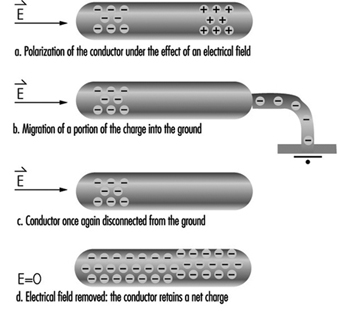
Hazards Associated with Static Electricity

The ill effects caused by the accumulation of static electricity range from the discomfort one experiences when touching a charged object, such as a door handle, to the very serious injuries, even fatalities, which can occur from an explosion induced by static electricity. The physiological effect of electrostatic discharges on humans ranges from uncomfortable prickling to violent reflex actions. These effects are produced by the discharge current and, especially, by the current density on the skin.

In this article we will describe some practical ways in which surfaces and objects can become charged (electrification). When the electrical field induced exceeds the ability of the surrounding environment to withstand the charge (that is, exceeds the dielectric strength of the environment), a discharge occurs. (In air, the dielectric strength is described by Paschen’s curve and is a function of the product of the pressure and the distance between the charged bodies.)

Disruptive discharges can take the following forms:

sparks or arcs which bridge two charged bodies (two metal electrodes)

partial, or brush, discharges which bridge a metal electrode and an insulator, or even two insulators; these discharges are termed partial because the conducting path does not totally short-circuit two metal electrodes, but is usually multiple and brushlike

corona discharges, also known as point effects, which arise in the strong electric field around small-radius charged bodies or electrodes.

Insulated conductors have a net capacitance C relative to ground. This relationship between charge and potential is expressed in equation 5 in table 1.

A person wearing insulating shoes is a common example of an insulated conductor. The human body is an electrostatic conductor, with a typical capacitance relative to ground of approximately 150 pF and a potential of up to 30 kV. Because people can be insulating conductors, they can experience electrostatic discharges, such as the more or less painful sensation sometimes produced when a hand approaches a door handle or other metal object. When the potential reaches approximately 2 kV, the equivalent to an energy of 0.3 mJ will be experienced, although this threshold varies from person to person. Stronger discharges may cause uncontrollable movements resulting in falls. In the case of workers using tools, the involuntary reflex motions may lead to injuries to the victim and others who may be working nearby. Equations 6 to 8 in table 1 describe the time course of the potential.

Actual arcing will occur when the strength of the induced electrical field exceeds the dielectric strength of air. Because of the rapid migration of charges in conductors, essentially all the charges flow to the discharge point, releasing all the stored energy into a spark. This can have serious implications when working with flammable or explosive substances or in flammable conditions.

The approach of a grounded electrode to a charged insulating surface modifies the electric field and induces a charge in the electrode. As the surfaces approach each other, the field strength increases, eventually leading to a partial discharge from the charged insulated surface. Because charges on insulating surfaces are not very mobile, only a small proportion of the surface participates in the discharge, and the energy released by this type of discharge is therefore much lower than in arcs.

The charge and transferred energy appear to be directly proportional to the diameter of the metal electrode, up to approximately 20 mm. The initial polarity of the insulator also influences charge and transferred energy. Partial discharges from positively charged surfaces are less energetic than those from negatively charged ones. It is impossible to determine, a priori, the energy transferred by a discharge from an insulating surface, in contrast to the situation involving conducting surfaces. In fact, because the insulating surface is not equipotential, it is not even possible to define the capacitances involved.

Creeping Discharge

We saw in equation 3 (table 1) that the surface charge density of an insulating surface in air cannot exceed 2,660 pC/cm².

If we consider an insulating plate or a film of thickness a, resting on a metal electrode or having one metal face, it is easy to demonstrate that the electrical field is drawn into the insulator by the induced charge on the electrode as charges are deposited on the non-metallic face. As a result, the electric field in the air is very weak, and lower than it would be if one of the faces were not metal. In this case, the dielectric strength of air does not limit charge accumulation on the insulating surface, and it is possible to reach very high surface charge densities (>2,660 pC/cm²). This charge accumulation increases the surface conductivity of the insulator.

When an electrode approaches an insulating surface, a creeping discharge involving a large proportion of the charged surface which has become conducting occurs. Because of the large surface areas involved, this type of discharge releases large amounts of energy. In the case of films, the air field is very weak, and the distance between the electrode and the film must be no more than the film thickness for a discharge to occur. A creeping discharge may also occur when a charged insulator is separated from its metallic undercoating. Under these circumstances, the air field increases abruptly and the entire surface of the insulator discharges to re-establish equilibrium.

Electrostatic Discharges and Fire and Explosion Hazards

In explosive atmospheres, violent exothermic oxidation reactions, involving energy transfer to the atmosphere, may be triggered by:

open flames

electric sparks

radio-frequency sparks near a strong radio source

sparks produced by collisions (e.g., between metal and concrete)

electrostatic discharges.

We are interested here only in the last case. The flash points (the temperature at which liquid vapours ignite on contact with a naked flame) of various liquids, and the auto-ignition temperature of various vapours are given in the Chemical Section of this Encyclopaedia. The fire hazard associated with electrostatic discharges can be assessed by reference to the lower flammability limit of gases, vapours and solid or liquid aerosols. This limit may vary considerably, as table 3 illustrates.

Table 3. Typical lower flammability limits

Discharge	Limit
Some powders	Several joules
Very fine sulphur and aluminium aerosols	Several millijoules
Vapours of hydrocarbons and other organic liquids	200 microjoules
Hydrogen and acetylene	20 microjoules
Explosives	1 microjoule

A mixture of air and a flammable gas or vapour can explode only when the concentration of the flammable substance is between its upper and lower explosive limits. Within this range, the minimal ignition energy (MIE)—the energy which an electrostatic discharge must possess to ignite the mixture—is highly concentration dependent. The minimal ignition energy has been consistently shown to depend on the speed of energy release and, by extension, on discharge duration. Electrode radius is also a factor:

Small-diameter electrodes (of the order of several millimetres) result in corona discharges rather than sparks.

With larger-diameter electrodes (of the order of several centimetres), the electrode mass serves to cool the sparks.

In general, the lowest MIEs are obtained with electrodes that are just big enough to prevent corona discharges.

The MIE also depends on the interelectrode distance, and is lowest at the quenching distance (“distance de pincement”), the distance at which the energy produced in the reaction zone exceeds the thermal losses at the electrodes. It has been experimentally demonstrated that each flammable substance has a maximum safe distance, corresponding to the minimum interelectrode distance at which an explosion can occur. For hydrocarbons, this is less than 1 mm.

The probability of powder explosions is concentration dependent, with the highest probability associated with concentrations of the order of 200 to 500 g/m³. The MIE is also dependent on particle size, with finer powders exploding more easily. For both gases and aerosols, the MIE decreases with temperature.

Industrial Examples

Many processes routinely used for handling and transporting chemicals generate electrostatic charges. These include:

pouring powders from sacks

screening

transport in pipework

liquid agitation, especially in the presence of multiple phases, suspended solids or droplets of non-miscible liquids

liquid spraying or misting.

The consequences of electrostatic charge generation include mechanical problems, an electrostatic discharge hazard for operators and, if products containing inflammable solvents or vapours are used, even explosion (see table 4).

Table 4. Specific charge associated with selected industrial operations

Operation	Specific charge (q/m) (C/kg)
Screening	10^-8 –10^-11
Silo filling or emptying	10^-7 –10^-9
Transport by worm conveyor	10^-6 –10^-8
Grinding	10^-6 –10^-7
Micronization	10^-4 –10^-7
Pneumatic transport	10^-4 –10^-6

Liquid hydrocarbons, such as oil, kerosene and many common solvents, have two characteristics which render them particularly sensitive to problems of static electricity:

high resistivity, which allows them to accumulate high levels of charges

flammable vapours, which increase the risk of low-energy discharges triggering fires and explosions.

Charges may be generated during transport flow (e.g., through pipework, pumps or valves). Passage through fine filters, such as those used during the filling of aeroplane tanks, may result in the generation of charge densities of several hundred microcoulombs per cubic metre. Particle sedimentation and the generation of charged mists or foams during flow-filling of tanks may also generate charges.

Between 1953 and 1971, static electricity was responsible for 35 fires and explosions during or following the filling of kerosene tanks, and even more accidents occurred during the filling of truck tanks. The presence of filters or splashing during filling (due to the generation of foams or mists) were the most commonly identified risk factors. Accidents have also occurred on board oil tankers, especially during tank cleaning.

Principles of Static Electricity Prevention

All problems related to static electricity derive from the:

generation of electric charges

accumulation of these charges on insulators or insulated conductors

electric field produced by these charges, which in turn results in a force or a disruptive discharge.

Preventive measures seek to avoid the accumulation of electrostatic charges, and the strategy of choice is to avoid generating the electric charges in the first place. If this is not possible, measures designed to ground the charges should be implemented. Finally, if discharges are unavoidable, sensitive objects should be protected from the effects of the discharges.

Suppression or reduction of the electrostatic charge generation

This is the first approach to electrostatic prevention that should be undertaken, because it is the only preventive measure that eliminates the problem at its source. However, as discussed earlier, charges are generated whenever two materials, at least one of which is insulating, come into contact and are subsequently separated. In practice, charge generation can occur even on contact and separation of a material with itself. In fact, charge generation involves the surface layers of materials. Because the slightest difference in surface humidity or surface contamination results in the generation of static charges, it is impossible to avoid charge generation completely.

To reduce the quantity of charges generated by surfaces coming into contact:

Avoid having materials come into contact with one another if they have very different electron affinities—that is, if they are very far apart in the triboelectric series. For example, avoid contact between glass and Teflon (PTFE), or between PVC and polyamide (nylon) (see table 2).

Reduce the rate of flow between materials. This reduces the shear velocity between solid materials. For example, one can reduce the flow rate of the extrusion of plastic films, of the movement of crushed materials on a conveyor, or of liquids in a pipeline.

No definitive safety limits for flow rates have been established. The British standard BS-5958-Part 2 Code of Practice for Control of Undesirable Static Electricity recommends that the product of the velocity (in metres per second) and the pipe diameter (in metres) be less than 0.38 for liquids with conductivities of less than 5 pS/m (in pico-siemens per metre) and less than 0.5 for liquids with conductivities above 5 pS/m. This criterion is valid only for single-phase liquids transported at speeds no greater than 7 m/s.

It should be noted that reducing shear or flow velocity not only reduces charge generation but also helps dissipate any charges that are generated. This is because lower flow velocities result in residence times that are higher than those associated with relaxation zones, where flow rates are reduced by strategies such as increasing pipe diameter. This, in turn, increases grounding.

Grounding of static electricity

The basic rule of electrostatic prevention is to eliminate the potential differences between objects. This can be done by connecting them or by grounding (earthing) them. Insulated conductors, however, can accumulate charges and thus may become charged by induction, a phenomenon which is unique to them. Discharges from conductors may take the form of high-energy—and dangerous—sparks.

This rule is consistent with recommendations regarding the prevention of electric shocks, which also require all accessible metal parts of electrical equipment to be grounded as in the French standard Low voltage electrical installations (NFC 15-100). For maximum electrostatic safety, our concern here, this rule should be generalized to all conducting elements. This includes metal table frames, door handles, electronic components, tanks used in the chemical industries, and the chassis of vehicles used to transport hydrocarbons.

From the point of view of electrostatic safety, the ideal world would be one in which everything would be a conductor and would be permanently grounded, thus transferring all charges into the earth. Under these circumstances, everything would be permanently equipotential, and the electric field—and the discharge risk—would consequently be zero. However, it is almost never possible to attain this ideal, for the following reasons:

Not all products which have to be handled are conductors, and many cannot be made conductive by the use of additives. Agricultural and pharmaceutical products, and high-purity liquids, are examples of these.

Desirable end-product properties, such as optical transparency or low thermal conductivity, may preclude the use of conductive materials.

It is impossible to permanently ground mobile equipment such as metal carts, cordless electronic tools, vehicles and even human operators.

Protection against electrostatic discharges

It should be borne in mind that this section is concerned only with the protection of electrostatically sensitive equipment from unavoidable discharges, the reduction of charge generation and the elimination of charges. The ability to protect equipment does not eliminate the fundamental necessity of preventing electrostatic charge accumulation in the first place.

As figure 2 illustrates, all electrostatic problems involve a source of electrostatic discharge (the initially charged object), a target which receives the discharge, and the environment through which the discharge travels (dielectric discharge). It should be noted that either the target or the environment can be electrostatically sensitive. Some examples of sensitive elements are listed in table 5.

Figure 2. Schematic of electrostatic discharge problem

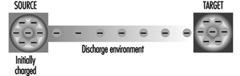
Table 6. Examples of equipment sensitive to electrostatic discharges

Sensitive element	Examples
Source	An operator touching a door handle or the chassis of a car A Charged electronic component coming into contact with a grounded object
Target	Electronic components or materials touching a charged operator
Environment	An explosive mixture ignited by an electrostatic discharge

Protection of workers

Workers who have reason to believe that they have become electrically charged (for example, when dismounting from a vehicle in dry weather or walking with certain types of shoes), can apply a number of protective measures, such as the following:

Reduce the current density at the skin level by touching a grounded conductor with a piece of metal such as a key or tool.

Reduce the peak value of the current by discharging to a dissipating object, if one is available (a table top or special device such as a protective wrist strap with serial resistance).

Protection in explosive atmospheres

In explosive atmospheres, it is the environment itself that is sensitive to electrostatic discharges, and discharges may result in ignition or explosion. Protection in these cases consists of replacing the air, either with a gas mixture whose oxygen content is less than the lower explosive limit, or with an inert gas, such as nitrogen. Inert gas has been used in silos and in reaction vessels in the chemical and pharmaceutical industries. In this case, adequate precautions to assure that workers receive an adequate air supply are needed.

Back

Published in 40. Electricity

Start
Prev
55
56
57
58
59
60
61
62
63
64
Next
End

Page 60 of 87

" DISCLAIMER: The ILO does not take responsibility for content presented on this web portal that is presented in any language other than English, which is the language used for the initial production and peer-review of original content. Certain statistics have not been updated since the production of the 4th edition of the Encyclopaedia (1998)."

More...

Contents